VVT26 - 2D conduction in cylindrical coordinate systems
| Solution | Test case |
|---|---|
| Case A | SVTEST257 |
| Case B | SVTEST258 |
Description
The purpose of this test case is to determine 2D conduction in circular pin fin using the finite element method. The steady-state temperatures predicted by the thermal solver are compared with the analytical solutions.
Geometry
To model the cylinder, the axisymmetric modeling technique is used, which requires a sketch on the XZ plane. A plate is sketched with a length of 1m and height of 0.75 m.
Simulation model
2D meshes are generated using axisymmetric parabolic quadrilaterals with an element size of 10 mm.
The following material properties are used:
- Material: Aluminum
- Thermal conductivity: k = 154.25 W/m·K
Two cases are studied:
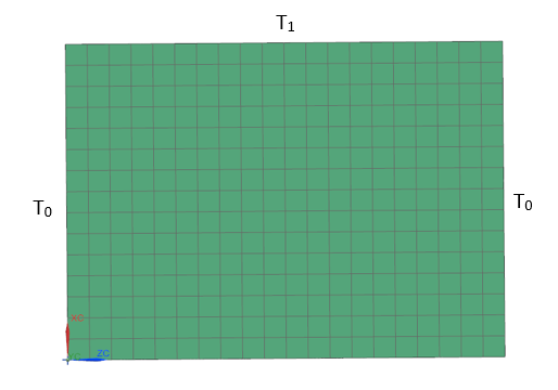
Case A: T =T(r,z) with a homogeneous z dimension
- Temperature constraint on the top edge of the fin with a value of T1 = 100 °C.
- Temperature constraint on the left and right edges of the fin with a value of T0 = 0 °C.
Case B: T =T(r,z) with a homogeneous r dimension
- Temperature constraint on the left edge of the fin with a value of T0 = 100 °C.
- Convection to Environment constraint on the top of the fin with a heat transfer coefficient h = 4113.33 W/m2 °C and a surrounding environment temperature T∞ = 20 °C.
Mesh and boundary conditions for case A

Mesh and boundary conditions for case B

This model uses the Multiphysics Thermal solution type with 2D Solid Option set to ZX Plane, Z Axis.
The default solver parameters are selected.
Theory
Case A solution for T=T(r,z) with homogeneous z dimension as follows:
where:
- I0 is the modified Bessel function of the first order.
- λn are the eigenvalues:
- Cn are the Fourier coefficients and defined as:
Case B solution for T=T(r,z) with homogeneous r dimension as follows:
where:
- Cn is defined as:
- λn are the roots of the following equation:
- J1 and J0 are the ordinary Bessel functions of order zero and order one, respectively.
- Bi is the Biot number.
Results
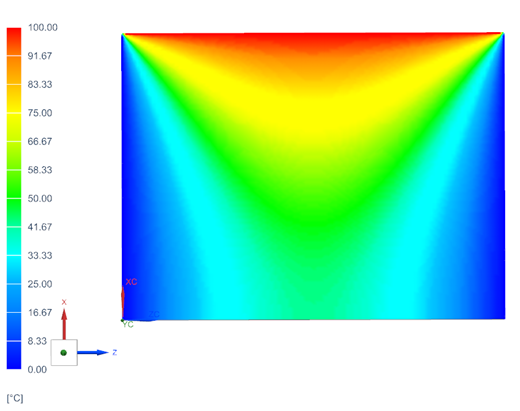
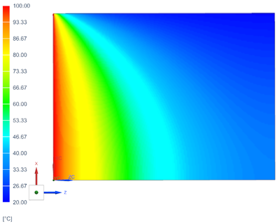
The following figures show the temperature distribution along the domain for case A and case B.
- Case A

- Case B

The following tables compare the computed temperature distribution obtained from theoretical calculation, with the nodal temperatures obtained from the thermal solver using the finite element method for:
- Case A
| Position (r, z) (m) | Ttheory (°C) | Tsim (°C) | Error (%) |
|---|---|---|---|
| (0.2, 0) | 25.589 | 26.04 | 1.76 |
| (0.2, 0.2) | 28.4031 | 28.9 | 1.75 |
| (0.2, 0.4) | 38.4831 | 39.09 | 1.58 |
| (0.2, 0.6) | 63.669 | 64.3 | 0.99 |
| (0.2, 0.7) | 86.4891 | 87.03 | 0.63 |
| (0.5, 0) | 42.9178 | 43.55 | 1.47 |
| (0.5, 0.2) | 47.0289 | 47.68 | 1.38 |
| (0.5, 0.4) | 59.8878 | 60.54 | 1.09 |
| (0.5, 0.6) | 81.4058 | 81.83 | 0.52 |
| (0.5, 0.7) | 93.7736 | 94.08 | 0.33 |
| (0.85, 0) | 19.8253 | 20.19 | 1.84 |
| (0.85, 0.2) | 22.0703 | 22.47 | 1.81 |
| (0.85, 0.4) | 30.3862 | 30.91 | 1.72 |
| (0.85, 0.6) | 54.2551 | 54.92 | 1.23 |
| (0.85, 0.7) | 82.124 | 82.27 | 0.18 |
- Case B
| Position (r, z) (m) | Ttheory (°C) | Tsim (°C) | Error (%) |
|---|---|---|---|
| (0.1, 0.2) | 86.1659 | 85.94 | 0.26 |
| (0.3, 0.2) | 62.094 | 61.55 | 0.87 |
| (0.5, 0.2) | 45.563 | 44.95 | 1.34 |
| (0.8, 0.2) | 33.4054 | 32.85 | 1.66 |
| (0.1, 0.6) | 71.9604 | 70.87 | 1.51 |
| (0.3, 0.6) | 42.2492 | 41.08 | 2.7 |
| (0.5, 0.6) | 31.1092 | 30.33 | 2.5 |
| (0.8, 0.6) | 25.1994 | 24.74 | 1.82 |
