Create thermal boundary conditions for an aeroengine compressor
Practice defining thermal boundary conditions for an axisymmetric aeroengine compressor. You will create thermal streams, voids, and convecting zones.
Open the Simulation file
Open the model Simulation file and reset the dialog box settings.
- Choose File→Open and open aeroengine/CompressorAxisymmetric_fem1_sim1.sim.
- Choose File→Preferences→User Interface and on the Dialog and Precision page, reset the dialog box memory.
- Click OK.
Explore the model
The Simulation file contains the Thermomechanical solution, which already has some thermal and structural boundary conditions defined. You will explore the predefined thermal contacts, loads, and temperature and convection constrains boundary conditions.
- In the Simulation Navigator, expand the Thermomechanical → Simulation Objects nodes to investigate the defined thermal contacts.
- Expand the Loads and Constraints nodes to investigate the predefined boundary conditions.
Create a thermal stream on edges
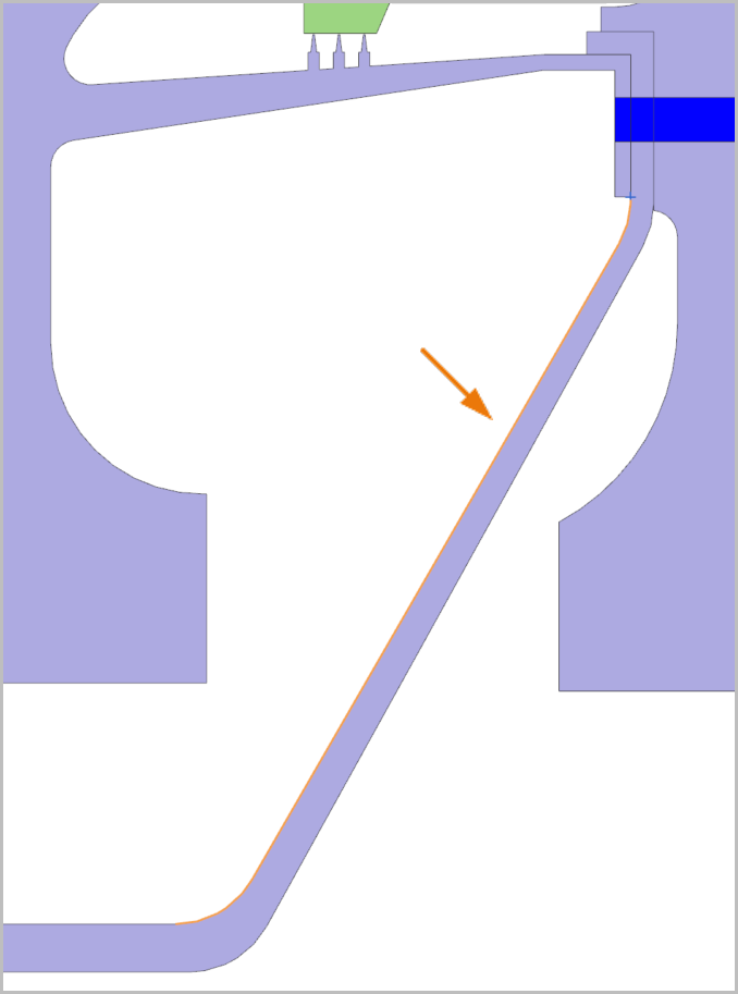
Create a thermal stream on edges using formulas and parameters to define their mass flow, inlet temperature, and pressure values to model the thermal effects of a fluid moving on the surface of engine components.
-
Choose Home tab→Loads and
Conditions group→Load Type
list→Thermal Stream
 .
.
-
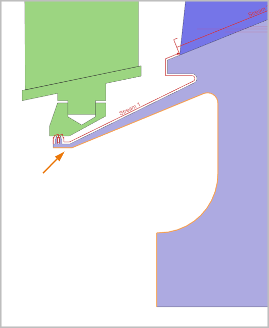
In the graphics window, select the edge (1). If the direction of the stream
is different than the direction shown in the image, click Reverse
Direction
 . Then select the edge (2) as
shown. The Method is automatically set to
Path Edges. This lets you select connected
edges.
. Then select the edge (2) as
shown. The Method is automatically set to
Path Edges. This lets you select connected
edges.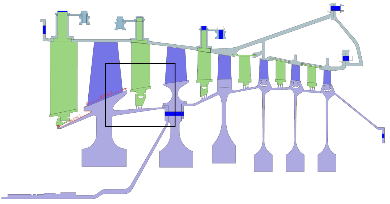
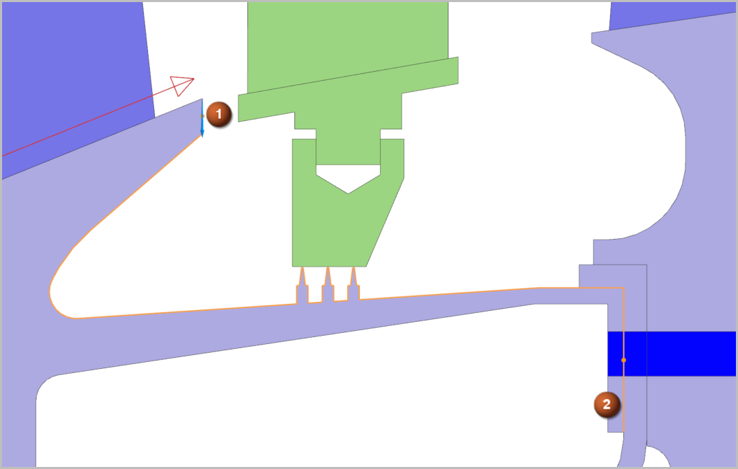
There are 22 selected edges. -
Set the following options:
- Fluid Materials=Air
- Mass Flow=SMO(2) kg/s
- Inlet Temperature=STO(2) °C
- Absolute Pressure=(1.2)*(P026+0.12*(P030-P026)) MPa
- Heat Transfer Coefficient=350 W/(m2·°C)
The mass flow and the inlet temperature are defined using an expression, which contain built in thermal-flow functions. The SMO(2) function returns the outlet fluid mass flow of the thermal stream with ID 2. The STO(2) function returns the outlet temperature of the thermal stream with ID 2. Pressure is defined with a formula, using the predefined parameters. To investigate these parameters, choose Menu → Tools → Expressions.
Note:Note: To define a magnitude using a formula, you can do one of the following:- Type the formula containing the parameters or functions in the magnitude box.
- Click
 to the right of the
magnitude box and choose:
to the right of the
magnitude box and choose:- Expression to define an expression using parameters.
- Function to find available functions and insert them.
Create a thermal stream on a face
Create a thermal stream on the compressor blade face to simulate fluid flow on the surface.
-
Select the blade face as shown.
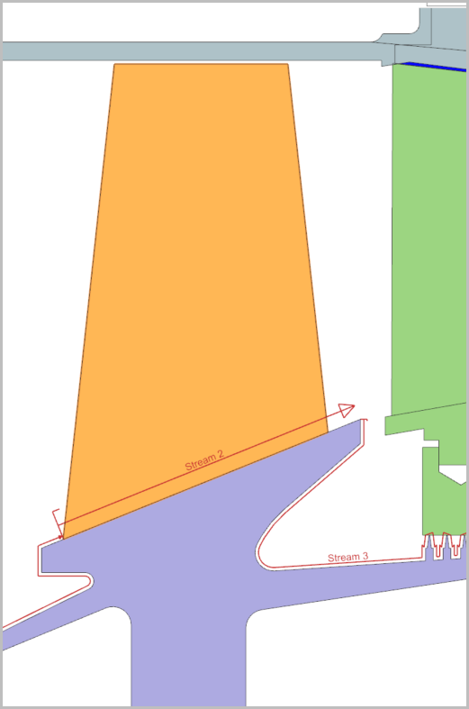
-
In the Direction group, from the Specify
Vector list, select XC-axis
 as the vector direction.
Create a thermal convecting zone
Define a thermal convecting zone that models convection for a specific fluid temperature.
-
Choose Home tab→Loads and
Conditions group→Simulation Object
Type list→Thermal Convecting Zone
 .
.
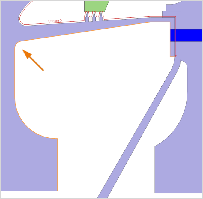
-
In the graphics window, select the 7 connected edges shown.
Create a thermal void
Create a thermal void that models regions that are in contact with a single fluid volume, such as a cavity, characterized by a single temperature and a negligible heat capacity.
-
Choose Home tab→Loads and
Conditions group→Simulation Object
Type list→Thermal Void
 .
.
-
In the Region 1 row, click Create
Region

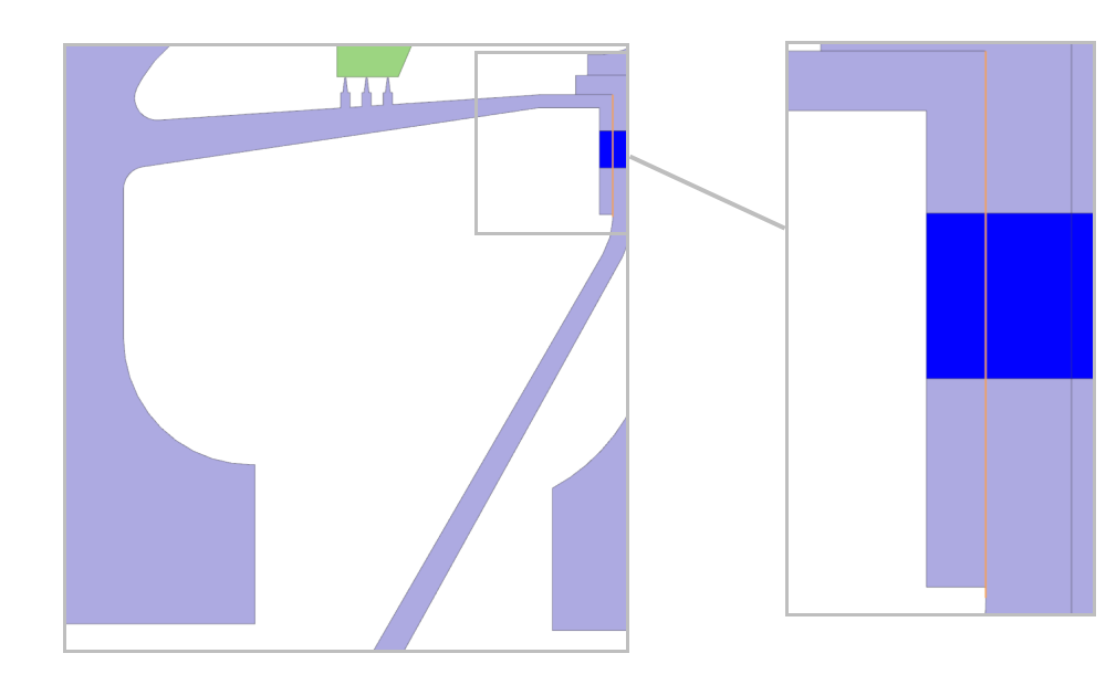
-
In the graphics window, select the 9 connected edges shown.
-
In the graphics window, select the shown edge.
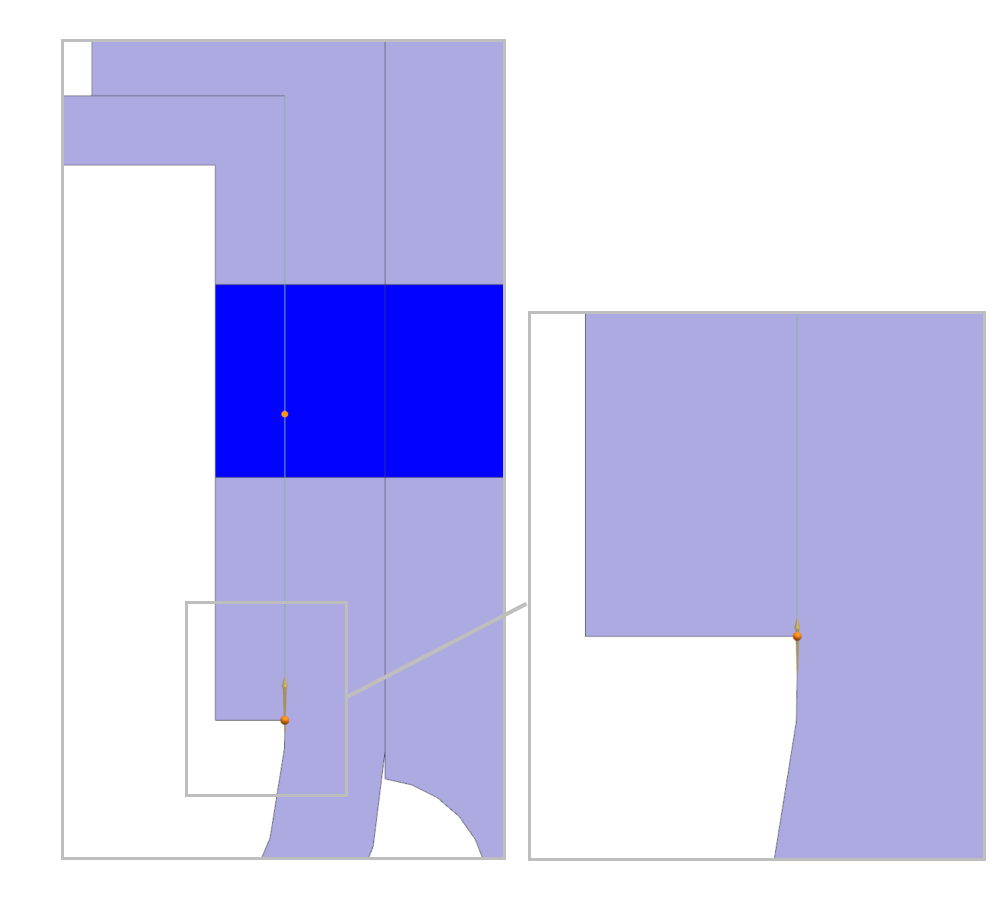
-
In the graphics window, select the end point as shown.
-
In the graphics window, select the 3 edges shown.
Solve the model
- In the Simulation Navigator, right-click the Thermomechanical node and choose Solve.
- Click OK.
- Wait for Complete to display in the Analysis Job Monitor dialog box, before proceeding.
- In the Review Results dialog box, click No.
- Close the Information window.
- In the Analysis Job Monitor dialog box, click Cancel.
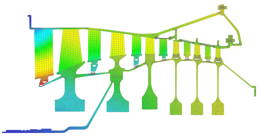
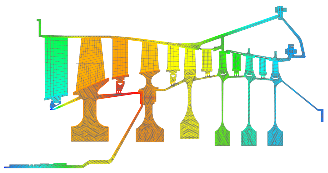
Display results
- In the Simulation Navigator, expand the Results node and double-click the Thermal node.
- In the Post Processing Navigator, expand the Thermal node and double-click the Temperature - Nodal node.
-
Choose Results tab→Post View
group→Edit Post View
 .
.
- In the Deformation tab, clear the Deformation check box.
- Click OK.
-
Expand the Post View 1 → Mesh
Collector nodes and clear the 0D
Elements check box.
- In the Post Processing Navigator, under the Thermomechanical node, right-click the Structural node and choose Load.
-
Expand the Structural → Increment
1,1.00s nodes and double-click
Displacement-Nodal.