Blade cooling
This topic explains why blade cooling is critical in gas turbines and how advanced cooling technologies allow turbine components to operate at temperatures above material limits.
This lesson may include hands-on exercises. Review the Discussion section for background information or click the button to proceed to the practical section.
Discussion
Blade cooling in turbomachinery allows modern gas turbines to operate at temperatures that exceed the melting points of the blade materials themselves. It works by bleeding cooler, compressed air through internal channels and expelling it over the exterior surfaces to create a protective thermal barrier.
Engine manufacturers use advanced cooling methods and ceramic thermal barrier coatings (TBCs) to maintain acceptable metal temperatures and extend component life.
Blade cooling is challenging because the flow and thermal fields inside a turbine are highly nonuniform. Heat transfer depends strongly on turbulence intensity, secondary flows, and local geometry effects. Simplified assumptions such as uniform flow or flat-plate boundary layers are therefore insufficient for accurate analysis.
- Blade cooling methods
- Blade cooling uses both internal and external cooling methods supplied by
compressor bleed air.
- Internal cooling removes heat through convection and impingement inside blade passages, evolving from simple single-pass channels to advanced multi-pass serpentine designs.
- External cooling includes film, transpiration, and effusion cooling. In film cooling, a common technique, a protective layer of air is generated between the hot gas-path flow and blade surface, by ejecting air out from the blade onto its surface.
Cooling is applied to critical regions such as the end wall, leading edge, trailing edge, and blade tip, where the tip experiences the highest thermal loads and requires the most effective cooling.
- Conjugate 1D flow
- Conjugate 1D flow modeling couples:
- A 3D solid thermal domain.
- A 1D flow domain.
This approach significantly reduces computational cost compared to full CFD while still capturing the thermal interaction between cooling flow and solid components.
The main gas path HTCs and temperatures can be approximated or mapped from external analyses.
Internal cooling flow can be modeled using:
- 1D ducts with thermal plugins.
- Immersed ducts.
- Co-simulation with external 1D flow solvers.
Conjugate 1D flow can be used with:
- Full 3D thermal models.
- Hybrid thermal-structural models.
- System-level thermal analyses.
This workflow is commonly used in industry because it balances accuracy and solution efficiency.
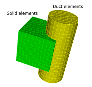
- Immersed ducts
- Immersed ducts model cooling channels using duct elements embedded inside a
3D solid mesh. The thermal solver automatically computes the thermal
coupling between the duct fluid and surrounding solid.
This method eliminates the need to explicitly mesh internal cooling passages in 3D, which significantly reduces:
- Model setup time.
- Mesh size.
- Computational cost.
Immersed ducts are supported by the finite-element thermal solver and can connect to standard 1D duct elements.
To compute convective heat transfer correctly, you must define the duct cross-sectional area. The solver uses this area to determine the convective coupling between the fluid and surrounding solid.
The thermal solver performs the following steps:
- Generates random points on the duct surface for each duct element.
- Detects intersections between the duct surface and surrounding solid elements.
- Computes a linear nodal distribution of convective area inside each solid element.
- Couples each solid element node with fluid element CG accounting for immersed area.
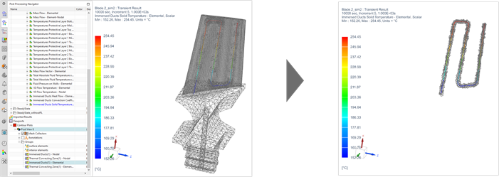
You can visualize which solid elements are thermally connected to immersed ducts during post-processing.
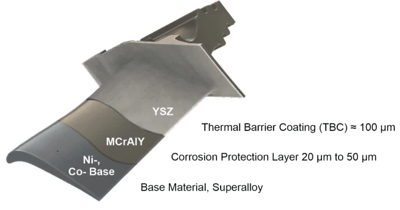
- Protective layers
- Hot-section blades and vanes commonly use thin ceramic thermal barrier
coatings (TBCs) to reduce metal temperature and improve durability.
Modeling these coatings presents several challenges:
- Very small layer thickness.
- Significant thermal resistance.
- Nonuniform thickness distributions.
- Difficulty meshing thin layers using standard meshing methods.
To address these challenges, the solver automatically generates thin prism layers on top of the solid surface mesh.
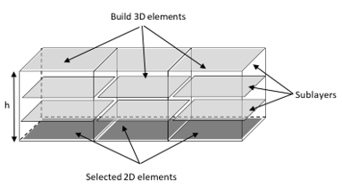
The solver:
- Creates a 3D mesh for each coating layer.
- Supports multiple sublayers.
- Allows field-defined thickness distributions.
- Automatically organizes layers into mesh groups for post-processing.
You can post-process temperatures at the bare-metal interface beneath the coating.
Use the Top Protective Layer Temperature result set to:
- Compare different coating thicknesses.
- Evaluate metal temperatures.
- Support coating design studies.
- Assess thermal protection effectiveness.
Hands-on material
To gain experience with the topics discussed here, complete the following: