Solving a model
This topic explains how to configure thermal-solver settings in WEM, including convergence criteria, discretization methods, integration methods, and axisymmetric-segment control for accurate and efficient thermal analyses.
This lesson may include hands-on exercises. Review the Discussion section for background information or click the button to proceed to the practical section.
Discussion
Use the Thermal Solution Control settings to define how the thermal solver advances the solution, evaluates convergence, and computes heat transfer.
- Convergence criteria
- Automatic defines default convergence criteria for the maximum temperature change between two consecutive iterations. This option is recommended for initial solution setup and first-pass analyses.
- Specify Max Temp Change defines the maximum allowable temperature change for any element between two consecutive iterations. When the temperature change for all elements falls below the specified value, the solver advances to the next time step.
- Iteration Limit defines the maximum number of iterations allowed before the solver advances to the next time step. The recommended range is 100-1000 iterations.
- Integration Method defines how the thermal solution advances in time. Use the Implicit integration method for most thermal analyses because it provides stable behavior for transient solutions.
- Element Discretization specifies the method for discretization of beam, shell, and solid elements when calculating element conductances. Finite Element Method is recommended for WEM and turbo applications.
- Conjugate Gradient Solver defines settings used to calculate convergence residuals during the linear thermal solve. If convergence difficulties occur, increase the Preconditioner Matrix Fill Value.
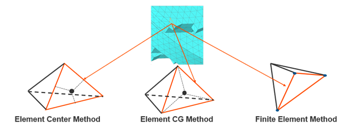
- Discretization methods in a thermal solution
- The thermal solver supports both finite-volume and finite-element
formulations. When the solver uses a finite-volume formulation, the element
nodes define only the element geometry. The numerical solution is computed
at control-volume locations rather than directly at the nodes.
The thermal solver supports the following discretization methods for conductive heat-transfer calculations:
- Element Center Method creates conductances
between element centers.
This method computes heat transfer using the centroid locations of neighboring elements.
- Element CG Method creates conductances
between the center of gravity (CG) of the element and surrounding
boundary elements.
This method provides an improved geometric representation compared to the simple element-center approach.
- Finite Element Method computes temperature
values directly at discrete nodal locations by solving the
heat-conduction equation.
The Finite Element Method is generally recommended for WEM analyses.
- Element Center Method creates conductances
between element centers.
- Number of axisymmetric segments
- The Number of Axisymmetric Segments parameter defines
how many radial segments the solver creates when revolving 1D or 2D
axisymmetric elements around the axis of revolution.
The thermal solver uses these revolved segments to generate a temporary 3D representation for radiation view-factor calculations when using the:
- Hemicube Rendering
- Deterministic
- Monte Carlo
Increasing the number of segments:
- Improves radiation view-factor accuracy.
- Provides better geometric representation of circumferential surfaces.
- Increases preprocessing and solution cost.
Note:This parameter affects not only radiation, but also the axisymmetric expansion of 1D fluid ducts. As a result, thermal coupling between fluid ducts and surrounding structures can be influenced by the selected number of segments.
Hands-on material
To gain experience with the topics discussed here, complete the following: