Define convection boundary conditions at 2D interfaces
Learn how to define thicknesses on 2D components and control thermal behavior at 2D interfaces. You will stitch interfaces, display free and stitched edges, apply thicknesses using expressions and specialized bolt/hole definitions, and validate areas used by the solver for convection and thermal couplings.
Introduction
Applying a mesh to a body is straightforward; however, defining thickness and controlling thermal behavior at 2D interfaces requires careful attention.
- Define thicknesses on various 2D components.
- Stitch interfaces in the FEM.
- Display and verify stitched edges.
- Apply thickness using expressions, bolt definitions, and hole definitions.
- Define Thermal Stream and Thermal Coupling boundary conditions.
- Evaluate the impact on conductive and convective areas.
- Verify the convective area used by the solver.
Define assembly load options
Load components from the same directory as the parent assembly.
-
On the Home tab, click Assembly Load
Options
 .
.
- From the Load list, select From Folder.
- Click OK.
Open the Simulation file
Open the simulation file and reset the dialog box settings.
- Choose File→Open and open thermal_bcs\HPC_sim.sim.
- Choose File→Preferences→User Interface and on the Dialog and Precision page, reset the dialog box memory.
- Click OK.
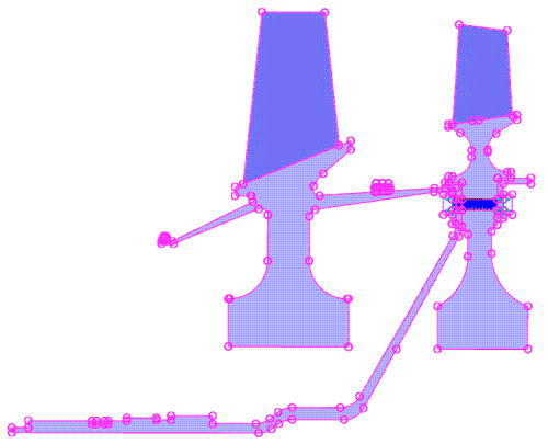
Display free and stitched edges
Open the workshop simulation and configure the display to review free edges and stitched edges.
-
Select Polygon Edges, then enable Display
Free Edges and Display Stitched
Edges.
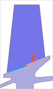
Free edges appear as pink lines. After stitching, internal edges appear as blue lines.
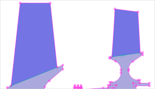
Stitch edges at the airfoil and disk interface
Stitch edges together at the base of the airfoil. In this case, thermal couplings between the blade and disk are not required, and convection boundary conditions can be applied to one internal edge, instead of two free edges.
-
Choose
 .
.
-
Select the polygon bodies of the disks and the blades at the airfoil and
disk interface.
-
Click OK.
Notice that internal edges between the airfoils and disks are highlighted in blue.
-
Choose
 to update meshes.
Apply thickness properties to the meshes
Apply thickness definitions to all plane stress regions and verify the results using thickness contours.
-
In the Simulation Navigator, right-click 2D Collectors
and choose Plot Thickness Contours.
This helps identify meshes with zero thickness regions.
Observe that four meshes have zero thickness and must be updated. Blade 1, blade 2, the bolt shank, and the bolt hole attached to disk 1.
-
In the Simulation Navigator, right-click
2D Collectors and choose Plot
Thickness Contours again to confirm thickness is defined for
all plane stress regions..
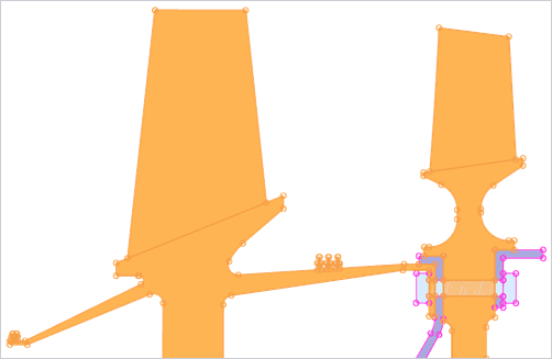
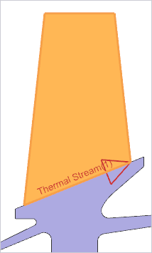
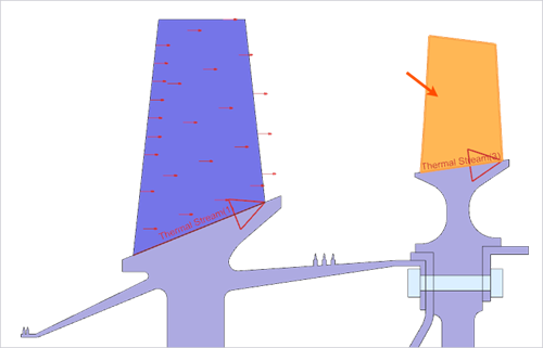
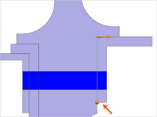
Apply thermal streams
Apply one-sided and two-sided thermal streams on internal edges, faces, and free edges, and control the convection area used by the solver.
-
Choose
 to apply a one-sided edge stream
on the internal edge of blade 1.
to apply a one-sided edge stream
on the internal edge of blade 1.
-
Select the shown edge.
Click Reverse Direction
 if the arrow orientation
does not match the direction shown in the image.
if the arrow orientation
does not match the direction shown in the image. -
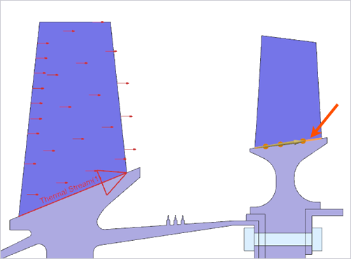
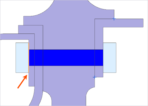
Apply a one-sided face stream to the face of the blade 1 in the Z-direction
as shown. Name the stream as
Blade1_airfoil_ID2.
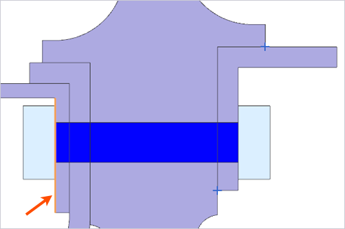
-
Apply a one-sided edge stream on the internal edge of the blade 2 as shown.
Name the stream as Blade2_root_ID3.
-
Apply a one-sided face stream to the face of the blade 2 in the
Z-direction. Name the stream as
Blade2_airfoil_ID4.
-
For the Side A:
- Select the four shown edges of the flange from the disk 3.
- Display the disk 2, and in the Path Limits
group, select Define Start Point, from the
list choose End Point and select the shown
edge to ensure the stream begins where the two components
interface.
- Select the four shown edges of the flange from the disk 3.
-
For the Side B:
- Select four edges of disk 2 as shown.
Hide the disk3 to ensure consistent edge selections for Side B.
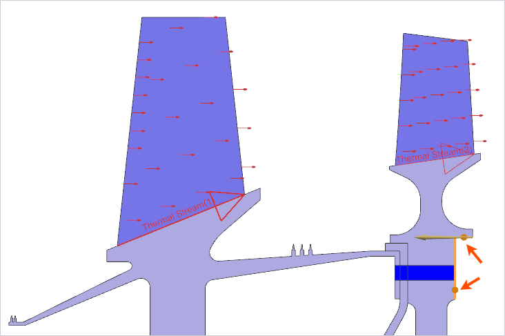
- Display the disk 3 and in the Path Limits
group, select Define End Point, from the list
choose End Point and select the shown edge to
ensure the stream ends at the inner radius of the disk 3
flange.
- Select four edges of disk 2 as shown.
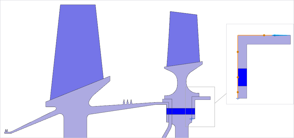
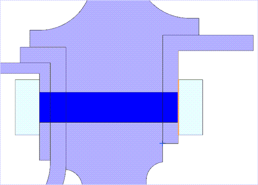
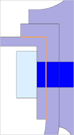
Apply the thermal contact between the bolt head and disk 1
Create the thermal coupling in the bolt head to the disk1 region.
-
Choose
 to define the contact between
the bolt head and disk 1 region.
to define the contact between
the bolt head and disk 1 region.
-
Display the three ROTOR_STAGE_2_BOLT components and
select the smaller region, consisting of the three edges of the bolt head,
as a primary region. For easier selection, hide the disk 1.
-
Select three edges of the disk 1, as a secondary region.
Tip: To focus on a specific polygon body during selection, expand the Body Focus group in the dialog box, click Select Body and select disk1 in the graphics window. Once selected, all other polygon bodies become temporarily translucent and unavailable for further selection.
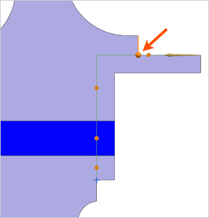
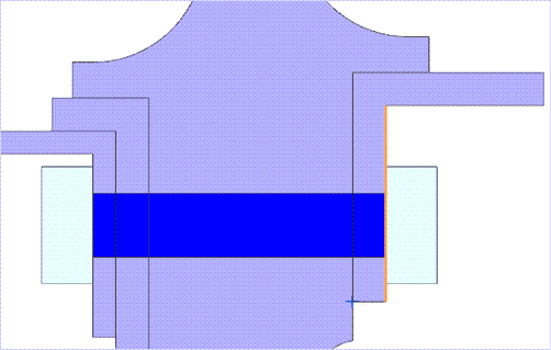
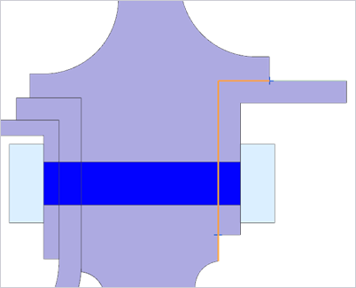
Verify solver-used areas
Validate the solver-used area when internal lines are present.
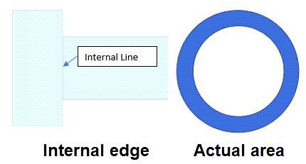
For regions like this, it is good practice to verify the area used by the thermal coupling to ensure accurate heat flow. Use the HPC_sim-Solution_1.bcdata file to identify the area calculated by the solver, then perform a hand calculation to confirm the correct contact area.
If you are using a version earlier than 2606, include the DISPLAY BC SUMMARY TABLES advanced parameter to write thermal and fluid properties of some boundary conditions in the file <simulation name>-<solution name>.bcdata.
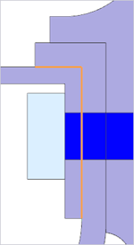
The image on the right shows the actual thermal contact area that should be used. For the contact between the bolt head and the disk 1, the correct area is:
mm2
-
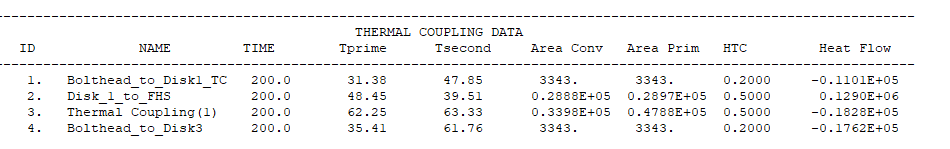
Open the HPC_sim-Solution_1.bcdata file and inspect
the reported area for the thermal coupling.
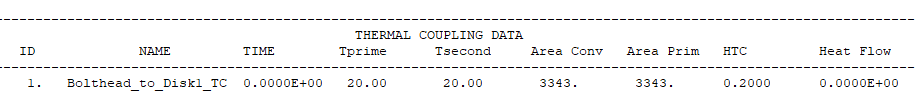
The convective area is calculated as 3343 [mm2].
The area correction factor for the HTC is
Since the solver-calculated area depends on mesh resolution and the correction factor is very close to 1, the area factor can be omitted for this thermal coupling.
Apply thermal contacts in the bolt head to disk 3, disk 1 to FHS, and disk 2 to disk 3
Create edge-to-edge contacts in the bolt head to disk 3, disk 1 to FHS, and disk 2 to disk 3.
-
For the Source Region, select the shown edge.
-
For the Target Region, select the shown edge.
-
Apply two additional thermal couplings using the process shown in the Apply the thermal contact between the bolt head and disk 1 with a Heat Transfer
Coefficient of 500 W/m2·°C.
Disk 1 to front hollow shaft (FHS) Disk 2 to disk 3 Primary region is the edge of the Disk 1.
Secondary region is the edge of the front hollow shaft.
Primary region is the edge of the Disk 3.
Secondary region is the edge of the Disk 2.
-
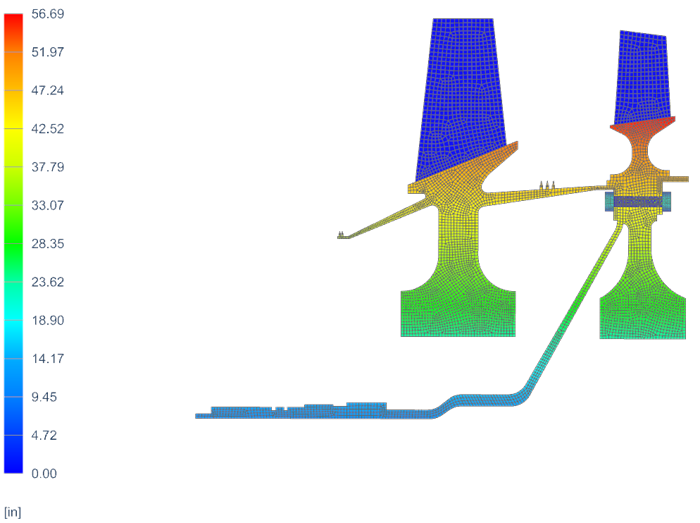
Solve the model and inspect the .bcdata.
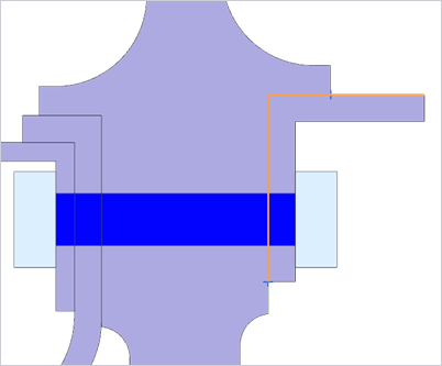
-
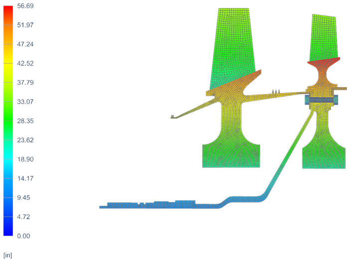
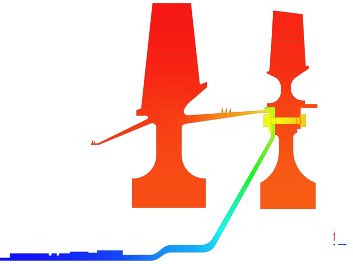
Inspect the temperature contours. The following image shows the nodal
temperature results at 5000s.
Additional notes
- Use the PLOT BC SUMMARY TABLES advanced parameters to review areas used in streams and thermal couplings.
- Pay special attention to convection areas on faces: solver-used area depends on mesh instance counts and any defined area factors or overrides.