Define convection boundary conditions using ducts
Learn how to model gas turbine thermal networks using a 1D duct approach.
Introduction
There are multiple approaches to modeling thermal networks in gas turbine engines. The appropriate method depends on the available input data, overall engine behavior, transient operating conditions, and engineering judgment.
In this tutorial, you will learn how to build a physics-based thermal model of a gas turbine using a 1D duct approach. You will:
- Set up a duct cooling network and model convection between ducts and components.
- Apply wall rotation and swirl ratio corrections to convective boundary conditions.
- Apply a heat load to account for windage heating.
- Reference duct outlet conditions within other boundary conditions.
- Post-process and validate key thermal results.
Load the thermal plugin
Enable the ExpressionsPlugin.dll if not already active. The predefined boundary conditions in the model use heat transfer coefficient (HTC) correlations implemented through custom expressions. These correlations require the plugin to evaluate correctly during the simulation.
- Choose .
- Click Simulation, expand Pre/Post, and scroll to Expressions.
- On the Plugin tab, select the Use Custom Plugin check box and in Custom Plugin, type the full path to the ExpressionsPlugin.dll file, as plugin\ExpressionsPlugin.dll.
- Click OK, exit Simcenter 3D, and restart the application to activate the plugin.
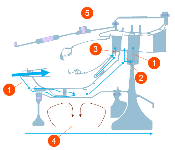
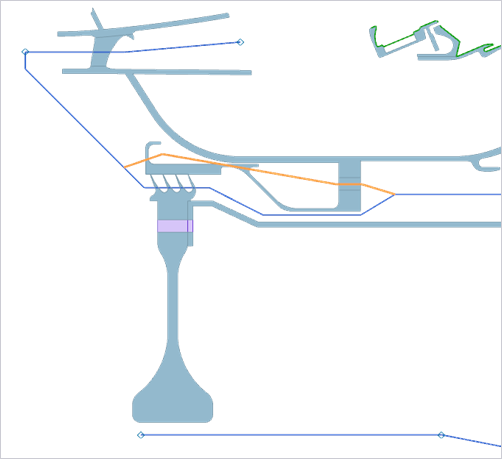
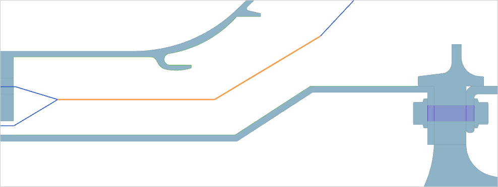
Understand flow directions
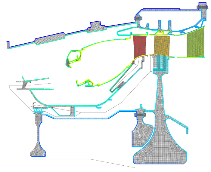
Review the cooling flow network and determine how thermal boundary conditions will be applied.
Understanding these flow features is essential before selecting and applying appropriate thermal boundary conditions.
-
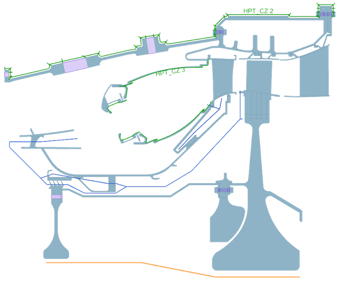
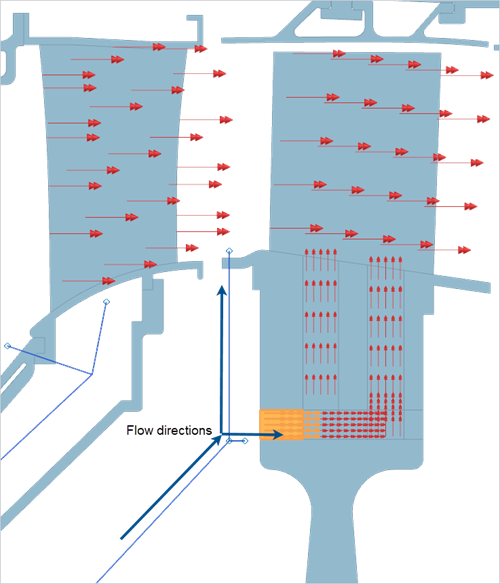
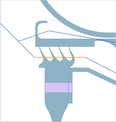
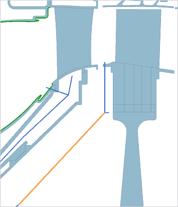
Review the provided flow schematic and identify blade cooling path (1)
flow, disk cavity purge flow (2), vane cooling flow (3), co-rotating
cavities (4) with no throughflow with unknown flow directions, and external
constant temperature regions (5).
-
Based on the identified flow directions and the available input data, the
following thermal boundary conditions are applied to represent the physics
of the system:
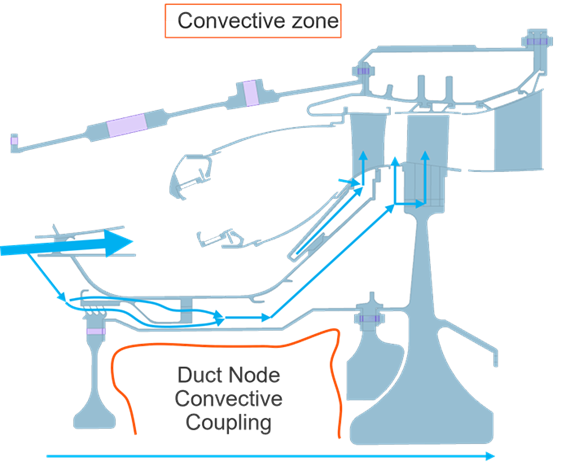
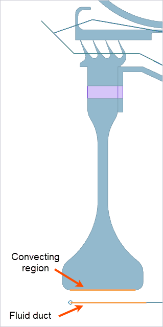
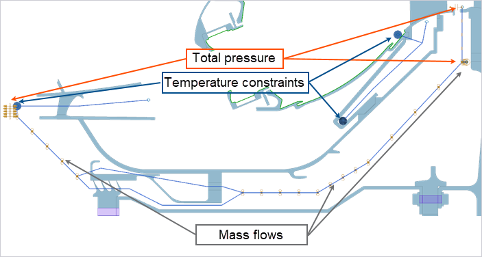
- An external Thermal Convecting Zone is defined to model heat exchange between the engine exterior and the surrounding environment.
- On the 1D ducts, the primary flow quantities are prescribed such as mass flow, total pressure, and inlet temperature.
- Thermal Coupling – Convection to connect the 1D fluid elements to the surrounding wall surfaces.
- Duct Node Convective Coupling in regions such as cavities where flow is assumed to be well mixed to connect a single duct node to multiple surrounding surfaces.
Apply the convective zone
Define the external engine convection using condition sequence parameters.
-
Choose
 to apply the convective
zone.
to apply the convective
zone.
-
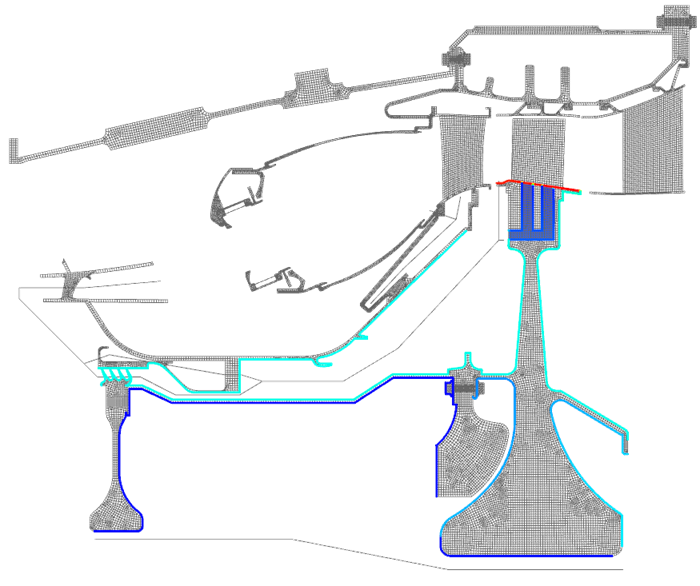
Select the external 32 edges as shown.

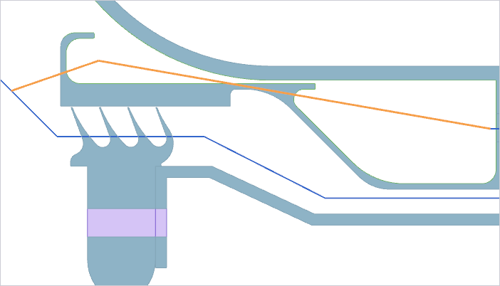
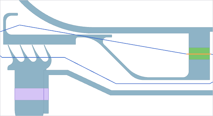
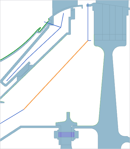
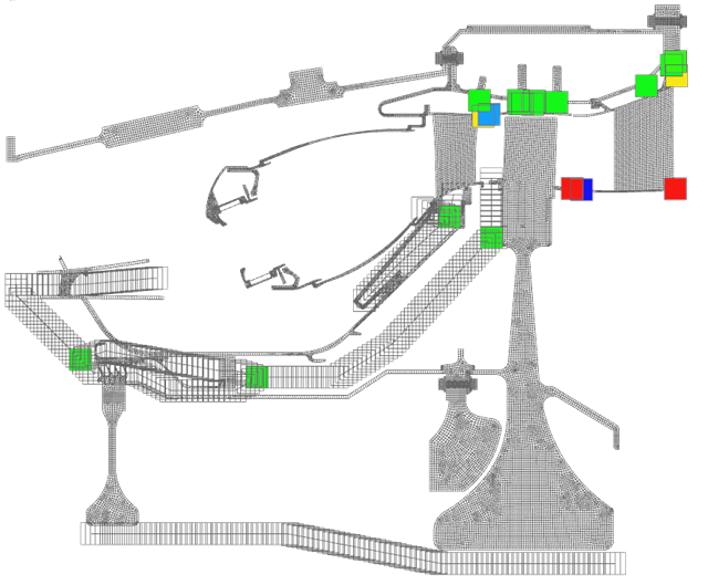
Setup the 1D duct network for secondary cooling flow
Define duct boundary conditions and convective couplings for the secondary cooling flow.
-
Press Ctrl+W and click Mesh Points to inspect node
locations.
Mesh points are used in the 1D duct network to maintain associativity when the fluid mesh is regenerated. If boundary conditions are applied directly to selected nodes and the model is re-meshed, those node selections may be lost, requiring all node-based boundary conditions to be redefined. Mesh points prevent this issue by forcing a node to be created at a specified location during meshing, ensuring consistent and robust boundary condition assignment.
-
Choose
 to define pressure for the secondary cooling
flow.
to define pressure for the secondary cooling
flow.
-
Select the following mesh point.
-
Apply the same duct boundary condition to the indicated mesh point, using a
pressure of 0.5*P26 MPa.
-
In the Simulation Navigator, click
 next to boundary conditions to
hide their display in the graphics window.
next to boundary conditions to
hide their display in the graphics window.
-
Choose
 to inspect the defined
conditions..
Because this is a transient analysis, certain quantities may need to be scaled using condition sequence parameters.
to inspect the defined
conditions..
Because this is a transient analysis, certain quantities may need to be scaled using condition sequence parameters. -
On the Parameters tab, press Ctrl, click
NH and SCALER, right-click
the selection and select Plot XY.
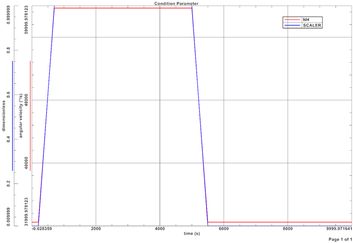
The SCALER parameter is a dimensionless quantity that scales from 0 to 1 based on speed. It can be used to scale quantities that are defined at full load or full power and need to be scaled through the transient cycle. -
Apply the Duct Fan/Pump type of the duct boundary
condition to the selected curves, and set the mass flow rate of
1*SCALER kg/s.
Note:The 1D element type Duct with Mass Flow Axisymmetric is used. This is the recommended duct type when importing results from an external 1D solver. It does not compute mass flow from pressure; the mass flow must be defined directly.For radiation and convection calculations, the axisymmetric elements are expanded circumferentially according to the Number of Axisymmetric Segments specified in Thermal Solution Parameters solver settings.
Increasing the number of segments can improve accuracy, but it also increases solution time.
-
Choose
 to define the inlet
temperature.
to define the inlet
temperature.
-
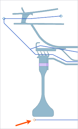
From the Selection Method list, select
Duct Fluid Nodes and select the shown node.
-
Select the shown edges.
-
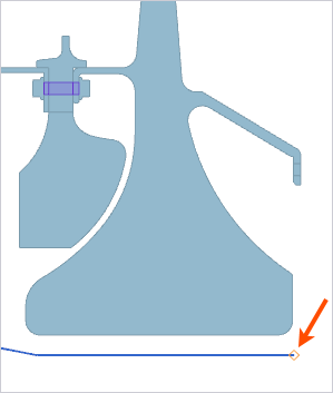
Apply convective coupling with the same settings to the shown edges:
-
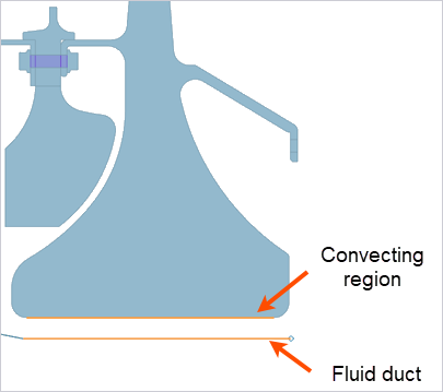
Select the shown 31 edges as convecting region, and shown node as a fluid
duct node.

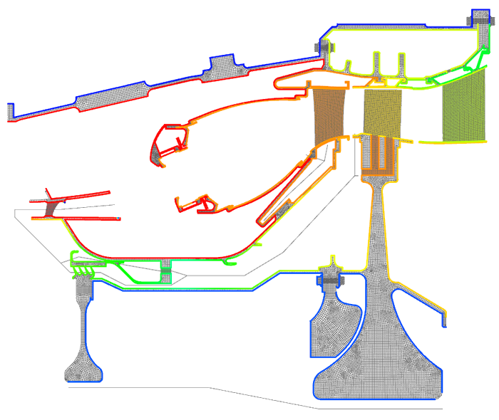
Setup the 1D duct network for blade cooling flow
Review the flow splits, define duct labels, and convective couplings for the blade cooling system.
-
Inspect the applied pressures, duct temperature constraints, and prescribed
mass flows on the duct elements as shown below. Note that a flow split
exists where the mass flow has not yet been defined.
-
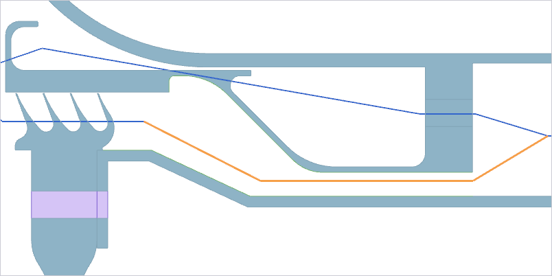
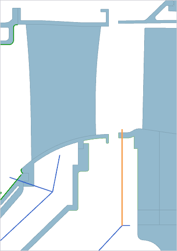
Inspect the flow direction for the shown ducts.
-
From the list, select Displayed.
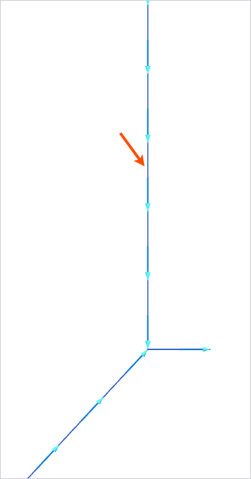
Notice that the displayed flow direction is incorrect. If this occurs, reverse the element direction in the FEM file to ensure the flow is oriented properly.
-
Apply a Duct Fan/Pump type of the duct boundary
condition to define a mass flow of 0.8*0.05*W26 kg/s
at the flow split as shown.
When the mass flow is defined in one branch, the mass flow in the other branch is automatically determined by conservation of mass.
-
In the Simulation Navigator, under
Loads, in the
HPT_StreamOnFace folder, right-click the
HPT_Stream 21 node and select
Edit to examine the flow split where part of the
supply air goes to the blade and part of the air purges into the flowpath.
Notice the use of DMO(), DTO(), and DPO() which allows you to connect
boundary conditions to ducts.
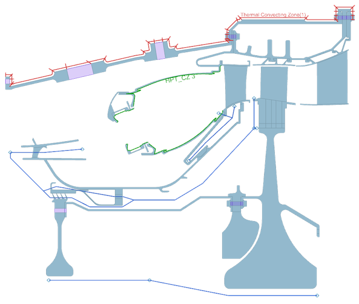
The following schematic shows flow directions.
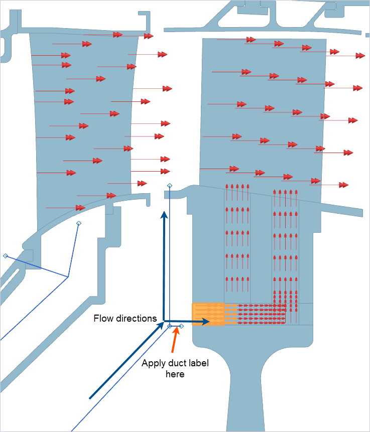
For this connection to work, a Duct Label type boundary condition is created on the 1D fluid mesh at the shown location, where data is to be extracted. The labeled location must be at a free end.
-
Choose to apply the following convective coupling for the blade
cooling.
These may use built-in correlations such as HTCFORCE or user-defined expressions. The inputs to these correlations do not always accurately represent the true geometry and often rely on simplified estimates of hydraulic diameter. The details of the built-in expressions can be reviewed in the Expression dialog box. In practice, users commonly develop their own custom expressions and reference them in the convective boundary conditions to better reflect the specific geometry and flow conditions.
- For the blade_supply_cc1 coupling,
select:Use the following settings:
Convecting Region (4 edges) Fluid Ducts (3 curves) 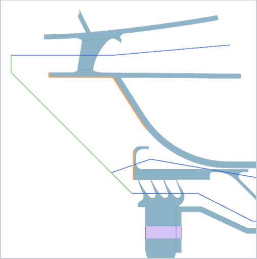

- Heat Transfer Coefficient = HTCFORCE(30[mm],"DUCT_FULL") W/m2·°C
- Only Connect Overlapping Elements is cleared
- For the blade_supply_cc2 coupling,
select:Use the following settings:
Convecting Region (22 edges) Fluid Ducts (1 curve) 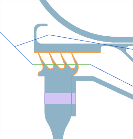
- Heat Transfer Coefficient = HTCFORCE(30[mm],"DUCT_FULL")
- Only Connect Overlapping Elements is cleared
- Rotational Effects = Correct for Wall Rotation
- Swirl Ratio = 0.55
- For the blade_supply_cc3 coupling,
select:Use the following settings:
Convecting Region (4 edges) Fluid Ducts (3 curves) 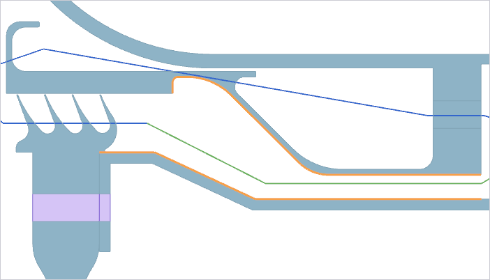
- Heat Transfer Coefficient = HTCFORCE(30[mm],"DUCT_FULL")
- Only Connect Overlapping Elements is cleared
- Rotational Effects = Correct for Wall Rotation
- Swirl Velocity = 0.55*nh*radius
- For the blade_supply_cc4 coupling,
select:Use the following settings:
Convecting Region (7 edges) Fluid Ducts (3 curves) 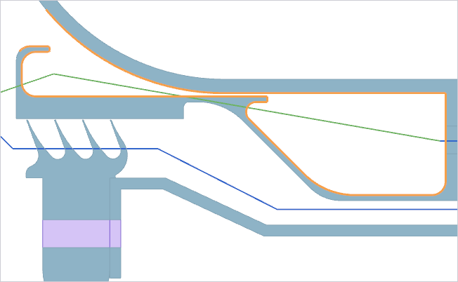
- Heat Transfer Coefficient = 100 W/m2·°C
- Only Connect Overlapping Elements is cleared
- For the blade_supply_cc5 coupling,
select:Use the following settings:
Convecting Region (1 face) Fluid Ducts (1 curve) 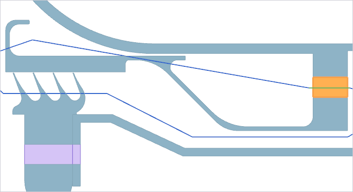
- Heat Transfer Coefficient = 6.35*PI()*10.99*20/6.35/11*100 W/m2·°C
- Only Connect Overlapping Elements is selected
When applying convective couplings to faces that represent holes or other plane stress regions, you must apply appropriate scaling factors to the heat transfer coefficient to ensure the correct convective heat transfer.
In this example, the HTC is defines as 6.35*PI()*10.99*20/6.35/11*100. This represents , where:
- HTC = 100
- For the blade_supply_cc6 coupling,
select:Use the following settings:
Convecting Region (11 edges) Fluid Ducts (2 curves) 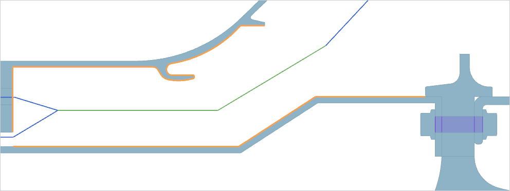
- Heat Transfer Coefficient = HTCFORCE(100[mm],"DUCT_FULL")
- Only Connect Overlapping Elements is cleared
- Rotational Effects = Correct for Wall Rotation
- Swirl Velocity = 0.5*nh*radius
- For the blade_supply_cc7 coupling,
select:Use the following settings:
Convecting Region (19 edges) Fluid Ducts (1 curve) 
- Heat Transfer Coefficient = HTCFORCE(30[mm],"DUCT_FULL")
- Only Connect Overlapping Elements is cleared
- Rotational Effects = Correct for Wall Rotation
- Swirl Velocity = 0.5*nh*radius
- For the purge_cc8 coupling, select:Use the following settings:
Convecting Region (16 edges) Fluid Ducts (1curve) 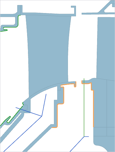
- Heat Transfer Coefficient = HTCFORCE(30[mm],"DUCT_FULL")
- Only Connect Overlapping Elements is cleared
- For the blade_supply_cc1 coupling,
select:
-
Choose to apply a heat load directly to the duct which will account
for windage rise in a rotor stator cavity.
Solve and post process
This model is configured for both thermal and structural analysis. However, since this activity focuses on the thermal setup, we will run the thermal solver only to reduce computational time. Solve and verify fluid temperatures, pressures, mass conservation, and applied heat loads.
-
In the Post Processing navigator, double-click
Thermal and expand and double-click Total Absolute Fluid Temperature
on Wall - Nodal at walls where wall rotation correction is
applied.
The temperature ranges from approximately 15 °C to 1626 °C.
-
Double-click Total Relative Fluid Temperature on Walls -
Nodal to display relative fluid temperature.
-
Double-click Fluid Pressure on Walls - Nodal to
display pressure on walls.
-
Inspect Mass Flow Junction Imbalance to confirm
conservation of mass.
If this value is non-zero, it indicates that mass is not conserved at a junction (for example, at a duct node connected to three elements).
Additional notes
- Thermal contacts are typically required in production models, though omitted here because this activity focuses on convective thermal boundary conditions.
- An alternative modeling approach uses streams and voids instead of explicit 1D ducts. In this approach, the thermal solver automatically generates the fluid elements used for convection, and the user connects the fluid network through junctions and expressions.
- When including radiation in axisymmetric models, use the Monte Carlo view factor method for improved accuracy.