Modeling the 1D duct network

Discussion

​There are two general approaches for modeling a 1D duct network:

1. Applying mass flows based on external 1D results.
2. Applying pressures based on external 1D results.

Use the Duct Flow Boundary Condition simulation object to model 1D duct network.

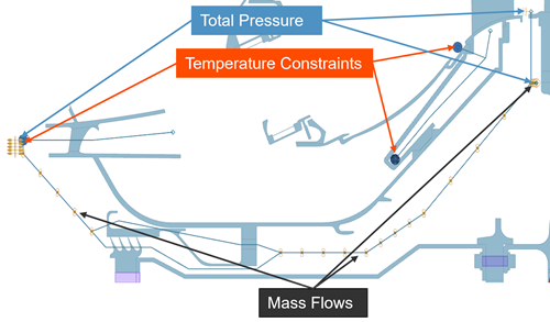
Applying mass flows based on external 1D results

​Use the following boundary conditions:

• Temperature constraint to define temperature at the nodes.
• Duct Total Pressure or Duct Static Pressure to define pressure at the nodes.
• Duct Opening to define pressure and temperature at the inlet or outlet of a duct network.
• Duct Fan/Pump to define mass flow in a duct network.

Tip:

It is recommended to use the Duct with Mass Flow or Duct with Mass Flow Axisymmetric physical property when meshing the ducts. If you use the Duct physical property, the model becomes over constrained, which will lead to unexpected results.

Comparing standard and axisymmetric ducts with mass flow

When modeling convective heat transfer in cyclically symmetric models or models that contain plane-stress or axisymmetric elements, you can use either Duct with Mass Flow or Duct with Mass Flow Axisymmetric. ​Both support cyclic symmetry, but the thermal solver computes heat transfer differently for each duct type.

Duct with Mass Flow

• Computes heat transfer directly using the 1D duct geometry and flow conditions.
• Does not expand the duct geometry circumferentially.
• Couples the cyclically symmetric solid segment directly to the 1D duct representation.

Duct with Mass Flow Axisymmetric

• Expands the duct geometry circumferentially around the axis of rotation.
• Computes heat transfer using the expanded axisymmetric representation.
• Couples the cyclically symmetric solid face to the expanded duct representation.

Solver treatment of duct with mass flow elements

Since no cross section is defined for 1D duct with mass flow elements, the thermal solver does not calculate pressure and fluid resistance. The thermal solver only calculates mass flow and temperature resulting from convection with the thermal elements.

• If a junction point has a remaining mass flow imbalance, the solver adds a compensating mass flow injection or loss at this junction.
• There is only convection through 1D duct with mass flow elements.

Comparing duct types

The following table compares standard mass flow ducts with axisymmetric mass flow ducts.

Aspect	Duct with Mass Flow	Duct with Mass Flow Axisymmetric
Coupling to cyclically symmetric body	Couples directly to 1D duct geometry	Duct expanded circumferentially and coupled
Mass flow interpretation	Total mass flow across all segments	Total mass flow across all segments
Typical use cases	3D cyclic symmetric bodies	Plane stress edges, axisymmetric edges
Mixed geometry support	Limited	Supports mixed geometries
Different segment counts	Not supported	Supported
When to use	Coupling to 3D cyclic symmetric bodies Geometry is fully 3D and symmetry is handled at the solid level	Coupling to plane stress edges Coupling to axisymmetric edges Connecting: Axisymmetric edges to 3D cyclic symmetric faces Cyclic symmetric bodies with different numbers of segments

Applying pressures at openings

Use the Duct Total Pressure to apply the total gauge fluid pressure at a point, mesh point, node, polygon edge, or curve within the duct network. The total pressure is the sum of static pressure and dynamic pressure. It applies pressure to all surfaces attached to selected ducts via Thermal Coupling - Convection.

It is recommended to select curves or polygon edges when you specify fluid pressure in a duct network because this allows you to retain the boundary condition selection when you remesh the model.

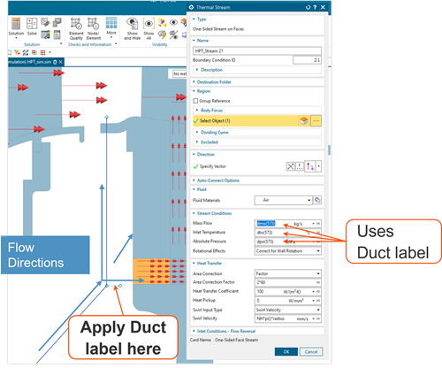
Assigning a boundary condition ID to the ducts

​Use the Duct Label type of Duct Flow Boundary Condition to assign a boundary condition ID to 1D duct curves/elements for reference in other boundary conditions using the following thermal-flow functions:

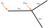
• DMO(i) returns the duct mass flow.
• DPO(i) returns the duct outlet pressure.
• DTO(i) returns the duct outlet temperature.

Where "i" is the duct label ID.

Defining thermal convection coupling

Convective thermal couplings model the convective heat transfer between a solid surface and a contacting fluid.

The convective heat transfer is defined as:

Use the Convection Coupling type of the Thermal Coupling - Convection simulation object to model convective heat transfer between the duct fluid elements and the convecting region.

Use the Duct Node Convection Coupling type of the Thermal Coupling - Convection simulation object to model convective heat transfer between the duct’s fluid nodes and the convecting region.

Both are similar to a stream or a void and include inputs for HTC and Total Temperature effects.

Considering adiabatic wall temperature for heat transfer

Use adiabatic wall temperature instead of the fluid temperature for heat transfer calculations in Thermal Convecting Zone and Thermal Coupling Convection to obtain accurate convective wall heat fluxes for flows with significant viscous heating such as high-speed flows in rotating and stationary machinery.

The thermal solver computes the wall heat flux as:

The adiabatic wall temperature T_aw on the stator side is:

The adiabatic wall temperature T_w on the rotor side is:

Where:

• is the recovery factor, which is calculated as:

  , where the Prandtl number is calculated at:

• is the heat transfer coefficient.
• is the wall temperature.
• is the adiabatic wall temperature.
• is the fluid temperature near the wall.
• is the fluid static temperature.
• is the specific heat of the fluid material at .
• is the relative tangential velocity, which is calculated as:

• is the swirl velocity.
• is the wall tangential velocity.

The Adiabatic Wall Temperature for Heat Transfer Calculations option is also available in Thermal Coupling – Convection and Duct Node Convection Coupling.

Hands-on material

To gain experience with the topics discussed here, complete the following:

• Define convection boundary conditions using ducts