Home
Turbomachinery getting started
This getting started guide provides a comprehensive introduction to thermal modeling for turbomachinery applications using Simcenter 3D Thermal Multiphysics.
Introducing boundary conditions
This topic explains the different types of boundary conditions used in turbomachinery simulations and how thermal, shared, and structural conditions are applied through simulation objects, constraints, and loads to represent multiphysics behavior.
Radiation modeling
This lesson explains the two Radiation simulation object types and how each defines radiative enclosures and affects radiation calculation efficiency.
Understanding radiation modeling with axisymmetric and plane-stress elements
This topic explains how the thermal solver models radiation in axisymmetric and mixed 2D axi-3D models, including transparency corrections and radiative behavior for plane-stress elements.

Knowledge base articles
Knowledge base articles provide concise, practical guidance for solving thermal, flow, multiphysics, space systems, and turbomachinery modeling challenges in Simcenter 3D.
Space thermal getting started
This getting started guide provides a comprehensive introduction to space thermal modeling using Simcenter 3D Space Systems Thermal (SST).
Turbomachinery getting started
This getting started guide provides a comprehensive introduction to thermal modeling for turbomachinery applications using Simcenter 3D Thermal Multiphysics.
- Getting started with turbomachinery in Simcenter 3D
- Fundamentals of turbomachinery systems
  This topic introduces turbomachinery and explains how gas turbines convert working-fluid energy into mechanical energy or thrust. You will learn how turbomachines are classified, how the Brayton cycle describes gas turbine operation, and how the main gas turbine sections, components, and cooling systems support safe and efficient performance.
- Gas turbine design disciplines and data exchange
  This topic introduces the main engineering disciplines involved in gas turbine design and explains how they exchange data throughout the development process. You will learn how different teams collaborate, what data they produce, and how iterative workflows drive the final engine design.
- Introducing Whole Engine Model (WEM)
  This topic introduces the WEM and explains its role in gas turbine design. You will learn how WEM captures the thermal and structural behavior of the engine, what inputs it requires, and how it supports clearance and mechanical integrity assessments.
- Introducing the user interface
  This topic covers the user interface (UI) in Simcenter 3D Thermal Multiphysics. You will learn how to navigate the modeling environment and how to efficiently use the available tools, menus, and commands to build, set up, and review your models.
- Preparing geometry for WEM
  This topic explains why geometry preparation is critical for WEM analysis. You will learn how to simplify 3D CAD geometry into efficient 2D or hybrid models and how to prepare geometry for meshing and simulation in Simcenter 3D.
- Meshing strategy
  This topic explains how to create finite element models for WEM by combining multiple mesh types and abstraction levels.
- Managing parts and assemblies
  This topic explains how to manage parts and assemblies in WEM using associative geometry, collaborative simulation capability, and integration of submodels into a full engine simulation.
- Condition sequences
  This topic explains how condition sequences define and manage engine operating conditions over a mission cycle in WEM.
- Introducing boundary conditions
  This topic explains the different types of boundary conditions used in turbomachinery simulations and how thermal, shared, and structural conditions are applied through simulation objects, constraints, and loads to represent multiphysics behavior.
  - Thermal coupling
    This topic explains how to model heat transfer between components that are not directly connected through the mesh in WEM simulations.
  - Convection boundary conditions
    This topic explains what thermal boundary conditions you can use for convection.
  - Fields, expressions and plugins
    This topic explains how to define boundary condition inputs in Simcenter 3D using fields, expressions, and plugin functions. These tools allow you to model complex, time- and space-dependent behavior efficiently.
  - Radiation modeling
    This lesson explains the two Radiation simulation object types and how each defines radiative enclosures and affects radiation calculation efficiency.
    - Understanding radiation modeling with axisymmetric and plane-stress elements
      This topic explains how the thermal solver models radiation in axisymmetric and mixed 2D axi-3D models, including transparency corrections and radiative behavior for plane-stress elements.
    - Radiation with cyclic symmetry
      This topic explains how the thermal solver handles radiation in sector models that use cyclic symmetry.
    - Strategies for radiation modeling in turbomachinery
      This topic provides general guidelines for selecting appropriate radiation modeling strategies in turbomachinery simulations.
  - Cyclic Symmetry
    This topic explains how to use Cyclic Symmetry in turbomachinery thermal models.
- Solving a model
  This topic explains how to configure thermal-solver settings in WEM, including convergence criteria, discretization methods, integration methods, and axisymmetric-segment control for accurate and efficient thermal analyses.
- Post-processing results
  This lesson introduces post-processing commands to help you review and evaluate simulation outcomes using visualization and data analysis.
- Mechanical integrity
  This topic explains how thermal results from WEM are mapped to detailed component models for structural and mechanical integrity analyses.
- Blade cooling
  This topic explains why blade cooling is critical in gas turbines and how advanced cooling technologies allow turbine components to operate at temperatures above material limits.
- Troubleshooting the model
  This topic explains how to verify FEM quality, material definitions, mesh integrity, and element properties before solving a thermal model.

Understanding radiation modeling with axisymmetric and plane-stress elements

This topic explains how the thermal solver models radiation in axisymmetric and mixed 2D axi-3D models, including transparency corrections and radiative behavior for plane-stress elements.

This lesson may include hands-on exercises. Review the Discussion section for background information or click the button to proceed to the practical section.

Discussion

For a model meshed with axisymmetric elements:

The thermal solver revolves the model around the axis of rotation to create a 3D representation.
Radiative view factors and conductances are computed as in a true 3D model.

For mixed 2D axi-3D models containing plane stress elements, the thermal solver uses a simplified axisymmetric radiation treatment, by creating axisymmetric elements with specific optical properties on top of the plane stress element edges.

In the following example, axisymmetric elements (in blue) created on top of the plane stress elements (in green) in 2D and 3D with external edge (1) and internal edge (2).

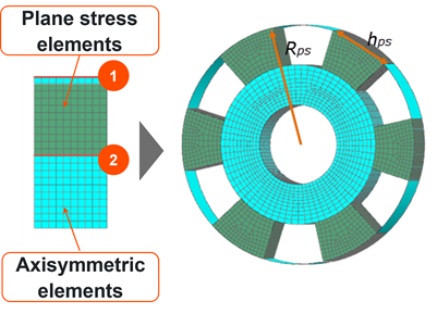
Mixed 2D axisymmetric–3D model showing plane-stress elements with simplified axisymmetric radiation treatment using axisymmetric radiation elements added along external and internal plane-stress edges.

Transparency correction for plane-stress elements

To account for partial circumferential coverage, the solver modifies the optical transparency, t, of the added axisymmetric elements:

Where:

is the radius of the top plane stress edges.
is the thickness of the top edge of the cyclic part meshed with plane stress elements.
is the number of instances of the cyclic parts.

The transparency factor, t, is a geometric scaling factor, not a material property.

The thermal solver renders plane stress elements semi-transparent or fully transparent depending on the origin of the ray.

If a ray travels from an external edge to an internal edge between axisymmetric and plane stress elements, the elements become semi-transparent.
If a ray travels from an internal edge to an external edge, the elements become fully transparent.

Hands-on material

To gain experience with the topics discussed here, complete the following: