Explore advanced thermo-optical properties for radiation modeling
Practice defining advanced thermo-optical properties for radiation modeling. You will troubleshoot issues associated with element normals and optical properties.
Open the model Simulation file
- Choose File→Open and open shellprops\shell_props_sim1.sim.
- Choose File→Preferences→User Interface and on the Dialog and Precision page, reset the dialog box memory.
-
Click OK.
The model consists of a wall mounted on a plate. It also contains a filament on one side of the wall, which is radiating a heat source emitting 200 Watts, and a box on other side. The model is meshed, and all the materials and properties are defined. The model contains two defined simulation objects:
- Radiative Heating to model a heat source.
- Enclosure Radiation to define physical enclosures within which the solver computes the radiation.
View the temperature results
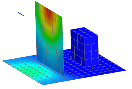
Verify that the heat distribution is correct from the beam elements emitting 200 Watts. You would expect the top section of the wall to have the maximum temperature as it is closer to the heat source.
- In the Simulation Navigator, expand Solution 1 → Results nodes, right-click the Thermal node and select Specify.
- In the Directory group, browse to the shellprops folder and select the .bun file.
- Click OK.
- In the Simulation Navigator, double-click the Thermal node.
-
In the Post Processing Navigator, expand the
Thermal node and double-click the
Temperature - Nodal node.
Notice that the hottest elements are not adjacent to the top wall, but on the base. In fact, the coldest elements are located near the top wall.
Examine the wall mesh collector
Examine thermo-optical properties and the element normals of the wall to verify that the wall side facing the heat source has appropriate thermo-optical properties.
-
Choose Home tab→Context
group→Return to Home
 .
.
- In the Simulation Navigator, right-click shell_props_fem.fem and choose Open in Window.
-
Expand the 2D Collectors node, right-click the wall node, and choose Edit.
Observe that the thermo-optical properties are only set for the top face. Only the top face of the wall models radiation. The top face of the wall is the face with positive normals.
- Click Cancel.
- In the Simulation Navigator, right-click the wall node and choose Check All → Element Normals.
-
Click Display Normals.
As suspected, the wall elements are facing away from the heat source. The filament is heating the bottom of the wall elements for which only thermo-optical properties are defined on top. You need to reverse the normals. -
Click Reverse Normals.
- Click Close.
Solve the model
Inspect warnings messages about the model that the Solution Monitor displays during the solution process.
- Click the (Simulation) shell_props_sim1.sim window to return to the simulation file.
- Right-click the Solution 1 node and choose Solve.
- Click OK.
- Wait for the solve to end, before proceeding.
- In the Review Results dialog box, click Yes.
-
Inspect the Simulation Monitor and locate the
WARNING message.
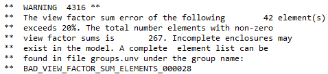
The warning message indicates that the radiation enclosure in the model is not complete. The next step shows how this affect the results. - Close Solution Monitor window.
- Close the Information window.
- In the Analysis Job Monitor dialog box, click Cancel.
View results on the corrected model
Review how your element normals correction influences the results.
- In the Simulation Navigator, double-click the Results node.
-
In the Post Processing Navigator, expand the
Thermal node and double-click the
Temperature - Nodal node.
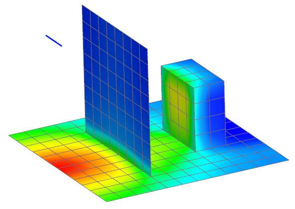
Now the results make more sense. The hottest temperature is on the wall, where the elements are closest to the beam elements. The coldest temperature is at the elements located furthest from the beam elements. Note that the wall is being heated by the filament, and it should also radiate to the box behind it. Observe that the block behind has no significant temperature change. The wall cannot radiate to the surfaces behind itself because its elements only have thermo-optical properties on the top side.
Import solution warnings
Import the solution warning groups that you inspected during the solution process.
-
Choose Home tab→Context
group→Return to Home
.
- Choose File tab→Import→Simulation.
- From the Select Solver list, select Simcenter 3D Thermal/Flow.
- Click OK.
- From the File Type list, select Solution Error/Warning Groups.
- In the Input File row, click Browse.
- Select the groups.unv file from the run directory.
- Click OK on both dialog boxes.
- Close Information window.
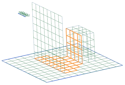
Evaluate failed elements
Observe the imported groups and analyze them.
Modify wall thermo-optical properties of the wall
Assign an emissivity of 0.8, an absorptivity of 0.05 to the top side of the wall, and an emissivity and absorptivity of 0.8 to the bottom side of the wall. You will set the top face transmissivity optical property to 0.95 and examine its effect.
- Switch to the (FEM) shell_props_fem.fem window.
- Right-click the wall node and choose Edit.
- In the Thermo-Optical Properties group, from the Radiation list, select Top and Bottom.
-
In the Top row, from the list, select Open Manager
 .
.
- From the Type list, select Thermo-Optical Properties-Advanced.
- In the Name box, type wall_top.
- Click Create.
- In the Infrared Properties group, in the Emissivity box, type 0.8.
- In the Solar Properties group, in the Absorptivity box, type 0.05.
- In the Transmissivity box, type 0.95.
- Click OK.
-
In the List group, click Add
 to add new thermo-optical properties to the list.
- Click Close.
- In the Bottom row, click Open Manager.
- From the Type list, select Thermo-Optical Properties-Advanced.
- In the Name box, type wall_bottom.
- Click Create.
- In the Infrared Properties group, in the Emissivity box, type 0.8.
- In the Solar Properties group, in the Absorptivity box, type 0.05.
- In the Solar Properties group, in the Transmissivity box, type 0.95.
- Click OK.
-
In the List group, click Add
to add new thermo-optical properties to the list.
- Click Close.
- Click OK.
Solve the improved model
- Switch to the (Simulation) shell_props_sim1.sim window.
- Right-click the Solution 1 node and choose Solve.
- Click OK.
- Wait for the solve to end, before proceeding.
- In the Review Results dialog box, click Yes.
- Inspect the Simulation Monitor and notice that the 4316 WARNING message has disappeared.
- Close the Information window.
- Click Cancel on the Analysis Job Monitor dialog box.
View results with transmissivity
View temperature results.
- In the Simulation Navigator, double-click the Results node.
-
In the Post Processing Navigator, expand the
Thermal node and double-click the
Temperature - Nodal node.
Observe that the temperatures still vary from 20 °C to 55 °C, however the temperature distribution on the face and the back box has changed. The radiation is now passing through the wall and heating the cube at the back.