Model radiation on 3D components
Model radiative heat transfer on 3D components and compare full radiation solutions with simplified approaches and evaluate solve time trade-offs.
Introduction
- Components have large temperature differences and they have a view factor with each other.
- Convection effects diminish, for example during shutdown when fluid flow throughout the engine decreases.
Typical regions in gas turbines include:
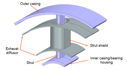
- The exhaust assembly, where hot diffusor walls radiate to cooler outer casings.
- The turbine inlet, where flowpath components are exposed to combustion gases or flame.
When modeling radiation, evaluate the following:
- Can you represent components with 2D elements?
- Can you apply cyclic symmetry?
- Can you divide the model into multiple enclosures to reduce solve time?
- Can you accept reduced accuracy to achieve significantly faster solve times?
In this tutorial, you will:
- Set up a radiation enclosure on 3D components.
- Evaluate methods to reduce radiation solve time.
- Inspect results and reports from a cyclic symmetry model with periodic radiation.
- Inspect results and reports from a cyclic symmetry model without periodic radiation.
- Build a simplified radiation model that solves quickly.
- Compare the results of different modeling approaches.
Load and inspect the model
Inspect components, identify radiating regions, and review boundary conditions.
-
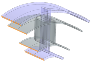
Inspect the geometry and identify major components of the 1/5 cyclically
symmetric sector.
-
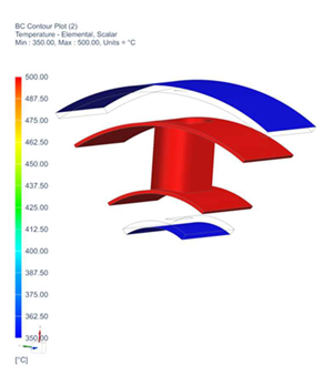
Select the temperature constraints, right-click the selection and select
Plot Contour to visualize the applied
temperatures.
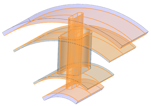
Create a Radiation Enclosure on 3D surfaces
Define a radiation enclosure using Monte Carlo view factor calculation.
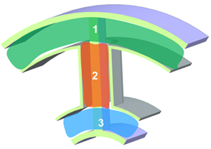
In this configuration, some surfaces in enclosure 1 would physically see surfaces in enclosures 2 and 3. However, dividing the model into separate enclosures eliminates many shadowing and visibility checks, which reduces computational cost but decreases physical accuracy.
-
Choose
 to define a single radiation enclosure for
maximum accuracy.
Use this approach when you need to compute view factors only once, extract them, and reuse them in subsequent analyses.
to define a single radiation enclosure for
maximum accuracy.
Use this approach when you need to compute view factors only once, extract them, and reuse them in subsequent analyses. -
For the Top Side Region, select the inside surfaces
of the casing, the outer surfaces of the diffusor, the strut, and the inside
of the strut shield.
34 surfaces are selected.
-
Next to Monte Carlo Settings, click
Edit
 and make sure that
Number of Rays is set to
2000.
You can increase the ray count if required until results converge within the required accuracy.
and make sure that
Number of Rays is set to
2000.
You can increase the ray count if required until results converge within the required accuracy.
Create a Cyclic Symmetry simulation object
Enable periodic radiation in a cyclic symmetry model.
-
Choose
 .
.
-
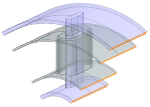
For the Source Region, select the shown faces.
-
For the Target Region, select the shown faces.
Apply Heat Map reports
Apply Heat Map reports to several regions where we are interested in view factors.
-
Choose
 .
.
-
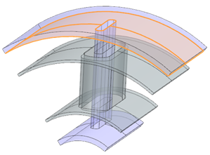
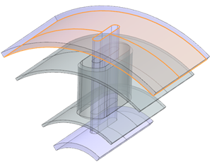
Select the shown faces.
-
Apply the following Heat Map reports.
Name Selection outer_diff 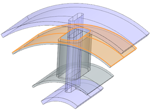
outer_strut 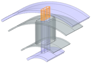
inner_case 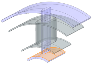
inner_diff 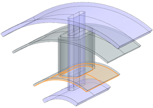
inner_strut 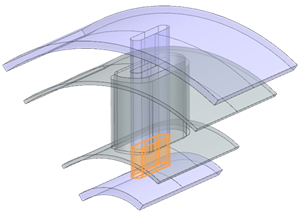
strut_shield 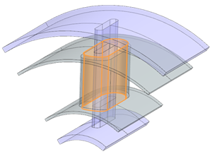
mid_strut 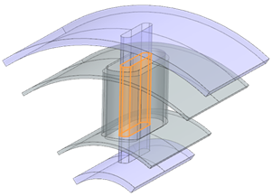
Solve a solution and inspect results
Inspect ther esults..
Apply radiation thermal couplings and solve the simplified radiation solution
Replace enclosure radiation with gray-body thermal couplings.
-
Choose
 .
.
-
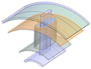
In the Primary Region group, select the shown
faces.
-
In the Secondary Region group, select the shown
faces.
-
Create another six radiation couplings based on dominant view
factors.
Primary Region Secondary Region Gray Body View Factor 0.433/5 0.221/5 2.274/5
3.506/5
0.514/5
0.845/5 Note:The emissivity of the mesh collector will be used in the radiation calculation along with grey body view factor to calculation radiative heat flow.
Use Result Probes to compare results
Compare full radiation, simplified radiation, and non-periodic radiation cases.
-
Choose
 to extract the averaged nodal temperature of
the strut region which is most influenced by radiation.
to extract the averaged nodal temperature of
the strut region which is most influenced by radiation.
-
Set the following:
- Load Case = All
- Selection Type = Nodes
- Select the strut region which is most influenced by radiation.

- Select the Combine Across Entities check box.
- Combined Value = Average
- Unit = °C
- Output Options = List
- Clear the Create Output check box
-
In the Post Processing Navigator, with one of the
graphs already displayed, press CTRL to select the two other graph items,
and choose Overlay.
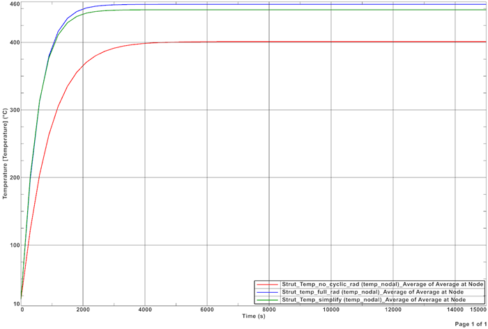
From these curves, the following conclusions are:
- The simplified radiation model predicts an average temperature within approximately 6 °C of the full radiation model at steady-state conditions.
- The close agreement between the full radiation model and the simplified model validates the use of gray body view factors and radiative conductances in the simplified approach.
- Disabling periodic radiation in the enclosure produces significantly different results, demonstrating that this approach does not adequately capture radiative behavior.
Additional Notes
- Avoid excessive heat map reports to reduce solve time.
- Review solve times:
- Radiation Enclosure with cyclic radiation: 26 hr 11 min
- Simplified radiation model: 4 min
- Radiation enclosure without cyclic radiation: 43 min