Define convection boundary conditions using thermal streams and voids
Learn how to model gas turbine thermal networks using thermal streams, voids, and convective zones.
Introduction
There are multiple approaches to modeling thermal networks in gas turbine engines. The appropriate method depends on the available input data, overall engine behavior, transient operating conditions, and engineering judgment.
In this tutorial, you will learn how to:
- Apply Thermal Stream, Thermal Void, and Thermal Convective Zone.
- Apply wall rotation and swirl ratio corrections to convective boundary conditions.
- Use the Auto-Connect stream option with a junction.
Load the thermal plugin
Enable the ExpressionsPlugin.dll if not already active. The predefined boundary conditions in the model use heat transfer coefficient (HTC) correlations implemented through custom expressions. These correlations require the plugin to evaluate correctly during the simulation.
- Choose .
- Click Simulation, expand Pre/Post, and scroll to Expressions.
- On the Plugin tab, select the Use Custom Plugin check box and in Custom Plugin, type the full path to the ExpressionsPlugin.dll file, as plugin\ExpressionsPlugin.dll.
- Click OK, exit Simcenter 3D, and restart the application to activate the plugin.
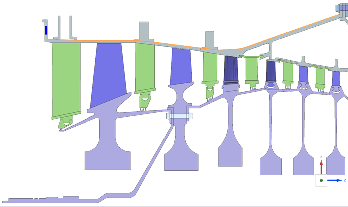
Define assembly load options
Configure search folders to load a model whose part and FEM files are stored in multiple directories.
-
On the Home tab, click Assembly Load
Options
 .
.
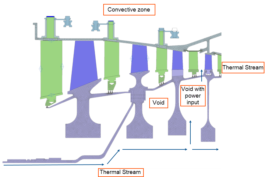
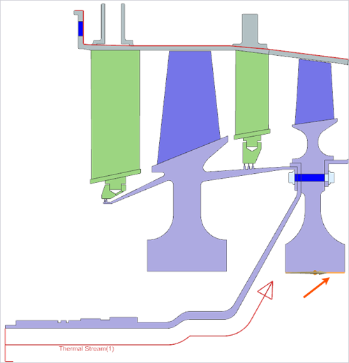
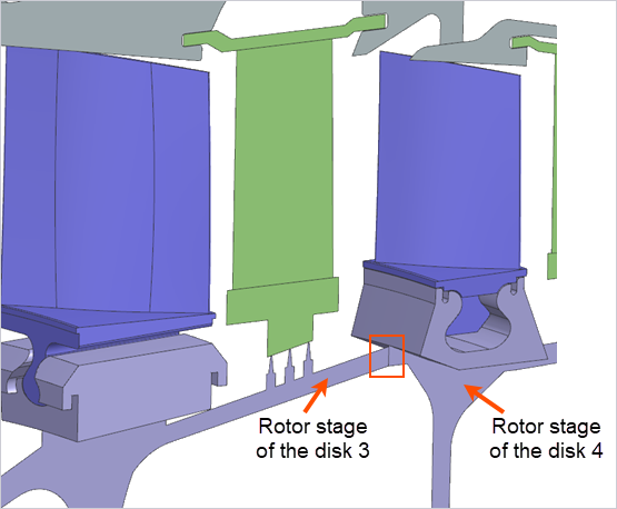
Understand flow directions
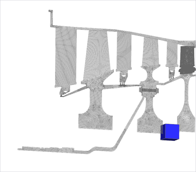
Review the cooling flow network before applying thermal boundary conditions. The direction and behavior of the flow depends on the data available to you. Typically, this information comes from a 1D secondary air system model and includes mass flow rates, pressures, temperatures, and swirl ratios.
-
Review the flow schematic and identify: dead cavities, rotor-rotor cavities
with leakage, and regions of constant external temperature.
- A dead cavity with no throughflow.
- A rotor-rotor cavity with a small amount of leakage passing through it, and there may be recirculating flows due to pumping effects.
- A constant air temperature at the exterior of the engine.
-
Apply the thermal boundary conditions as outlined below, based on the
identified flow directions and available data. For simplicity in this
tutorial, constant values will be used for the convective heat transfer
coefficients. In practice, it is recommended to use appropriate correlations
such as HTCFORCE, or functions implemented through
custom thermal plugins to obtain more realistic results.
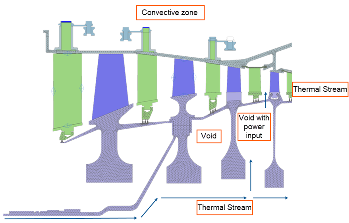
Apply the thermal convective zone
Define external convection using condition sequence parameters.
-
Choose
 to apply the convective
zone.
to apply the convective
zone.
-
Select the external 18 edges as shown.
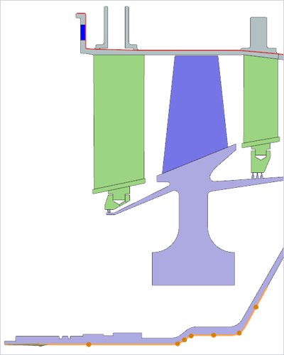
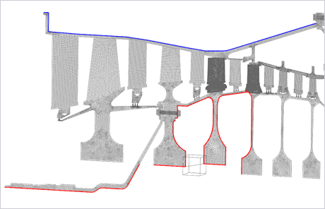
Apply thermal streams
Create one-sided and connected streams, reference upstream conditions, and apply wall rotation corrections.
-
Choose
 to apply a one-sided edge
stream.
to apply a one-sided edge
stream.
-
Select the shown 7 edges.
-
Create another thermal stream as shown.
-
Create a third stream as shown.
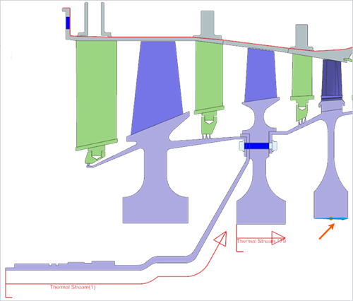
Make sure that the direction of the stream as shown. If needed, click Reverse Direction.
-
Choose
 to connect thermal stream 179 to
the stream 180.
to connect thermal stream 179 to
the stream 180.
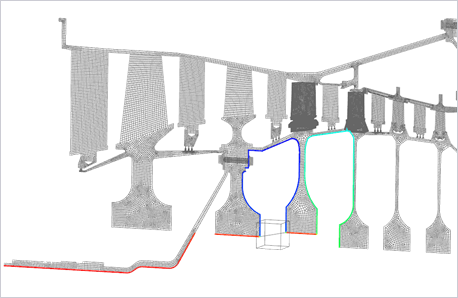
Apply thermal voids
Define cavity regions and account for heat exchange using void boundary conditions.
-
Choose
 to create a void region in the first
cavity.
to create a void region in the first
cavity.
-
In the Regions 1-5 group, click Create
Region
 and select the shown 11
edges.
and select the shown 11
edges.
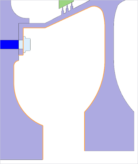
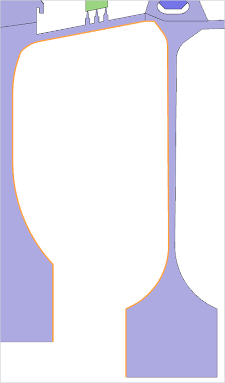
If different heat transfer coefficients are required within the void, define multiple regions to assign separate HTC values accordingly.
-
For the region, select the following 9 edges and apply the same settings as
for the previous void, except set the pressure to
sp(180).
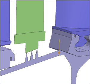
Apply stream for the leakage air
Model leakage convection using a two-sided edge stream.
-
Apply a two sided edge stream to model convection of the leakage air on the
highlighted edges.
Two sided is required here because there are two free edges at this interface. If an internal edge were used by stitching the edges, using a single sided edge stream with the Add thickness option would be appropriate.
-
Make sure that the direction of the stream as shown in the image.
Solve and post process
Validate fluid temperatures, pressures, and mass conservation.
-
In the Post Processing navigator, expand the and double-click Total Absolute Fluid Temperature
on Wall - Nodal.
-
Double-click Fluid Pressure on Walls - Nodal at
walls where wall rotation correction is applied.
-
Double-click Mass Flow Junction Imbalance to verify
conservation of mass.
If this magnitude is non-zero, this means mass has not been conserved at the junction between streams.
Additional notes
- The Automatically Connect option works for junctions and for streams that geometrically share endpoints.
- Thermal contacts are typically required in production models but were omitted here to focus on convective boundary conditions.
- An alternative approach is to mesh 1D ducts and use Thermal Coupling – Convection to connect ducts to component surfaces.