Set up a hybrid 2D and 3D thermal model
Practice setting up and solving a hybrid thermal model that consists of the 2D axisymmetric part and 3D repetition part of the cyclic symmetric geometry.
Open the Simulation file
Open the Simulation file and reset the dialog box settings.
-
Click OK.
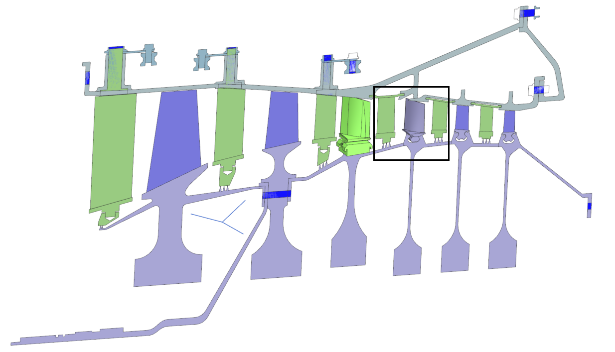
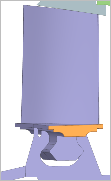
The model consists of 2D parts for most of the compressor and 3D parts for rotor stages 3 and 4. The model is meshed and all the material and properties are defined. All the boundary conditions are defined in the model except for the rotor stage 4. The solution is created from the condition sequence and contains eight steps.
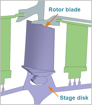
Connect the 2D and 3D parts of the rotor stage 4
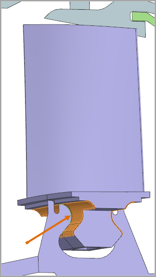
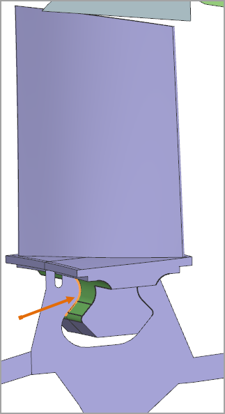
Model conduction between the disk and blade of rotor stage 4 using thermal coupling.
- In the Simulation Navigator, under the Solution 1, expand Simulation Objects, right-click the 2D-3D node and choose New Simulation Object → Thermal Coupling.
- In the Name group, type Stage_4_2D_to_3D.
-
For the primary region, select 6 polygon faces. Three on one side, and
three on the opposite side. These faces contact with the 2D part.
-
For the secondary region, select 4 edges of the 2D part. Two edges on one
side, and two on the opposite side. Tip: Use filter Polygon Edge.
- In the Magnitude group, from the Type list, select Heat Transfer Coefficient.
- In the Coefficient box, specify 1000 W/(m2·°C).
- In the Additional Parameters group, make sure that the Only Connect Overlapping Elements check box is selected.
- Click OK.
Define two-sided stream on face and edge
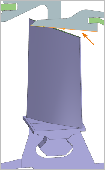
Define a stream at the tip of the 3D blade with two-sided stream on edges and faces.
-
Right-click the Stream on Face-Edge node and choose
New Load → Thermal Stream
 .
.
-
In the graphics window, select the edge of the 2D part.
Make sure the stream direction is from left to right. If not, click Reverse Direction
 .
.
-
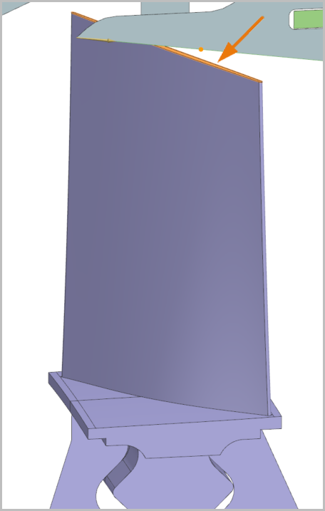
In the graphics window, select the polygon face.
Tip: Use filter Polygon Face.
-
In the Simulation Navigator, next to
Simulation Objects and
Loads, click
 to hide the nodes.
Define Cyclic Symmetry for the blade
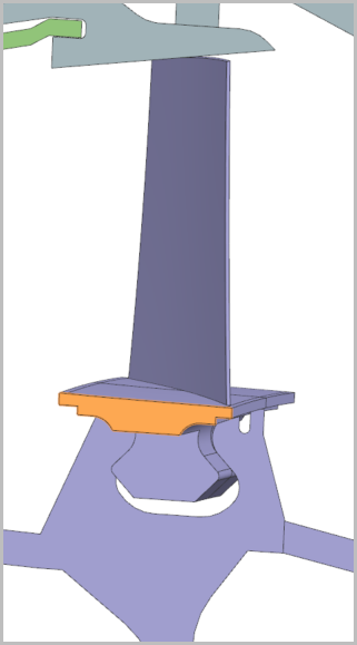
Define the Cyclic Symmetry boundary condition to scale the material and convective areas to consider the number of blades.
-
Right-click the 2D-3D node and choose New
Simulation Object → Cyclic Symmetry
 .
.
-
In the Source Region group, click Create
Region, rotate the model if needed, and select the displayed
polygon face.
-
Rotate the model and select the opposite polygon face.
-
Click CSYS Dialog
 .
.
Connect the created stream with existing streams
Create junction connections between streams.
-
Right-click the Junctions node and choose
New Simulation Object →
Junction
 .
.
- In the Incoming Streams group, select Stream 35 from the Stream 1 list and Stream 34 from the Stream 2 list.
- In the Outgoing Streams group, select Stream 36 from the Stream 1 list.
- Click OK.
Solve the model
Solve the model and monitor its completion.
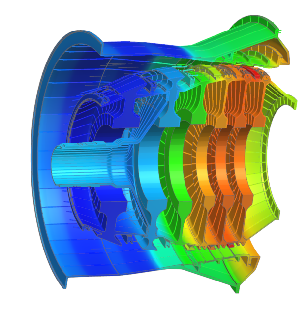
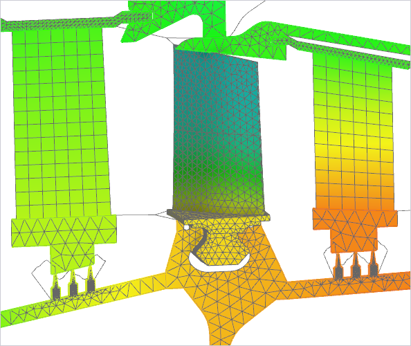
Display temperature results
Display temperature results.
- In the Post Processing Navigator, double-click the Thermal node to load the results.
- Expand Thermal→ Time 2000.0 → Increment 1, 2.000E+03s → Temperature - Nodal.
-
Expand the Post View 1 → Mesh
Collector node, and clear the OD
Elements check
box.
-
Choose Results tab→Animation
group→Animate
 .
.
- From the Animate list, select Iterations.
-
Click Play
 , then
Stop
, then
Stop
 .
.
- Click Close.
Display axisymmetric results
Display results for axisymmetric elements as a 3D model using Axisymmetric Options.
- In the Post Processing Navigator, right-click the Post View and choose Edit Result.
- In the Coordinate System group, select Absolute Cylindrical from the list.
- In the Symmetric Result Options group, click Set Symmetric Results.
- From the Display list, select 3D Model.
- Click OK.
-
Choose Results tab →
Display group →
Feature
 .
.
-
Choose Results tab →
Display group → Cutting Plane
Options
 .
.
-
In the Cut Direction group, from the
Axis list, select YC
 .
.
-
In the Cut Position group, select the
Apply Immediately check box.