How to generate reduced thermal models in Simcenter 3D
This article explains how to generate a reduced thermal model (RTM) in Simcenter 3D.
What is a reduced thermal model?
A reduced thermal model is a simplified representation of a thermal system that preserves key thermal behavior while reducing computational effort. It consists of a simplified geometry containing only the external components called the geometrical mathematical model (GMM), and non-geometric thermal network representing the internal components, called the thermal mathematical model (TMM).
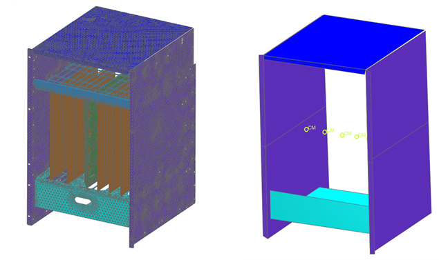
The following example illustrates the detailed FEM and RTM.
- Contains fewer nodes and elements.
- Preserves the dominant heat transfer characteristics such as conduction, convection, and radiation.
- Runs faster compared to the full model.
- Full-scale thermal simulations are too time or resource consuming.
- You need to translate the model to other thermal software.
- You need to test multiple configurations.
- Select zones.
- Generate the TMM, using one of the following methods:
- PARAM REDUCE advanced control
- Gebhardt method
- Generate the GMM.
- Compare results and validate the models by comparing the INPF.reduced file data from the full and reduced models.
- Use TMG Correlation to tune the values that match your target.
- Use the reduced model with Thermal Exchanger to run a simulation in Ansys Thermal Desktop™ or run different configurations to identify the best design, or export the model to other software using STEP-TAS.
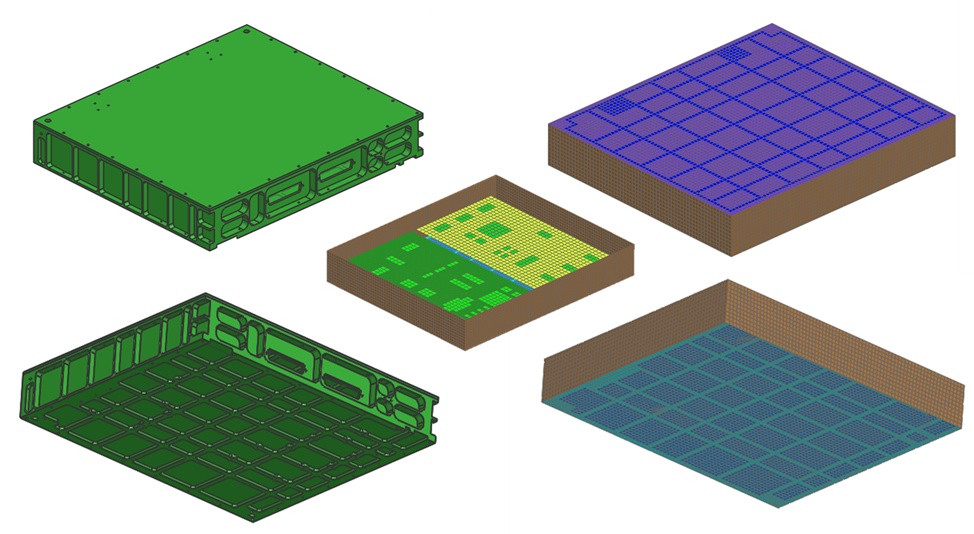
The electronic unit model that includes two PCBs, various electronic components, and a supporting structure is used to illustrate how to reduce the model.
Selecting zones
Reducing a thermal model involves merging zones to decrease the element count. When merged, all elements in a zone share a single temperature, thermal capacitances and dissipations are combined, and thermal couplings to neighboring zones are recalculated. The method used to define zones and compute couplings depends on the chosen TMM approach.
In Simcenter 3D, you create zones based on isothermal zones or based on your knowledge of the system and the expected temperature gradients. You identify the temperatures from a simulation, split the elements by temperature ranges, and generate corresponding groups. To accelerate the process, you can write a script to automate it.
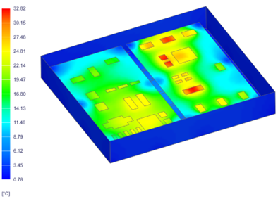
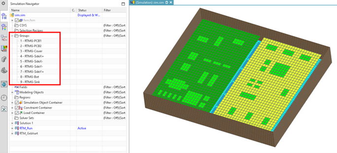
The following example shows multiple PCB zones in the RTM.
- Keep the temperature gradient within the group small.
- Group components that share a heat load.
- Avoid referencing the same element in multiple groups.
- Ensure all elements interacting with reduced parts have their own group.
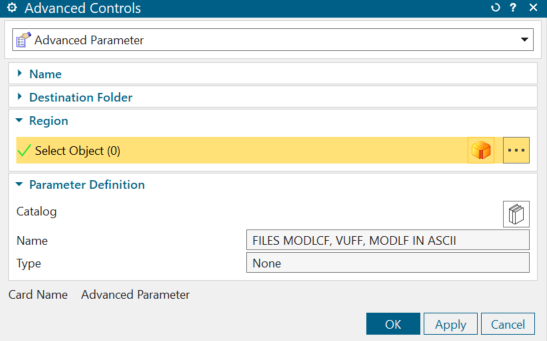
- Convert the output files to the ASCII format. In the solution, that is used
to generate zones, define the FILES MODLCF, VUFF, MODLF IN ASCII advanced
parameter in the Advanced Controls simulation
object.
- Define groups to be reduced independently to have more control over the
process.
- Run the simulation.
- Open the TEMPF file, which contains the temperatures of all elements, filter
by temperature ranges, and generate corresponding zones.
- If you create groups in step 2, a script can be created to automate the process to organize the file by groups. You can find the list of element IDs in each group in the INPF file in the run directory.
- Apply a temperature threshold to each group. Start from the minimum or maximum temperature and divide the group into temperature ranges.
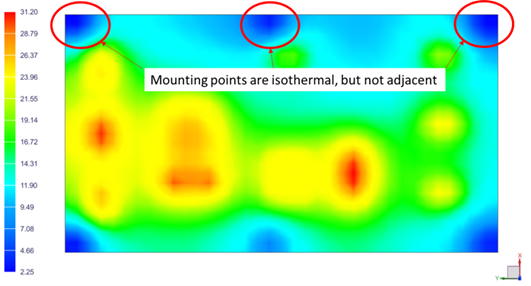
- After filtering, you may notice that some isothermal zones within a
group are not adjacent. If needed, you can subdivide these into
separate zones by ensuring that only elements with shared nodes
belong to the same zone. The INPF file contains the node list for
each element, which can be used to enforce this criterion.
- Import the zones into the model to facilitate the following steps. Format the elements list into a groups.unv file. To import the groups, click , select the Simcenter Thermal/Flow solver, in the File Type list, select Solution Error/Warning Groups.
- Merge the zones by using the Merge Set simulation object if the TMM is generated with the Gebhardt model.
Generating the thermal mathematical model
Once the zones are generated, calculate the equivalent thermal conductances between them. This article provides two methods, each with its own advantages and limitations. The choice depends on the specific requirements of the application.
Using PARAM REDUCE
This method is easy to use but has a key drawback: conductances are computed from temperatures rather than the model’s geometrical and thermal properties. The software calculates conductive and radiative heat flows between zones and divides them by the temperature difference or energy difference for radiative couplings. While physically valid, the results are affected by numerical approximations. Small temperature gradients can lead to large variations in conductance values. In transient simulations, conductances change over time, making them dependent on the specific boundary conditions of the simulation used to generate the TMM, which limits RTM accuracy.
- Thermal nodes definition.
- Heat loads (QNODE).
- Initial temperatures (TINIT).
- Element capacitances (XCAP) for each group.
- Conductive conductances (XCOND COND) between groups.
- Radiative conductances (XCOND RAD) between groups.
- Correspondence between the element labels of the full and reduced model. It will be deleted during the generation of the GMM.
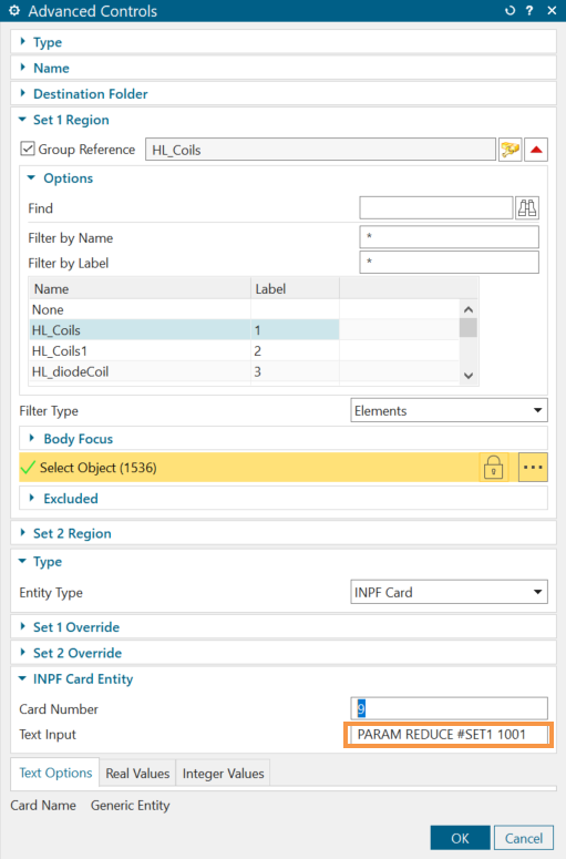
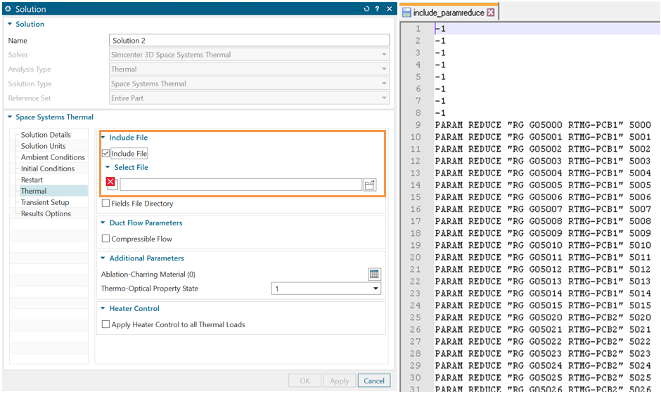
- In the Set 1 Region, select the defined zone.
- In INPF Card Entity, set the Card Number to 9.
- In Text Input, enter PARAM REDUCE #SET1 ID, where
#SET1 references the selected group in Set 1 Region,
and ID is the user-defined identifier assigned to the selection in
Set Region 1, which the software writes to the
INPF.reduced file to make it easier to locate.
- T1: group of elements, which is a zone. T1 is the name of the group of elements to be condensed to the single thermal node T2.
- T2: thermal node label.
- T3: optional parameter to recover temperatures.
Using the Gebhardt method
This method uses the geometric and thermal properties of the model to compute the equivalent conductances between groups. Since the values are not determined based on temperatures, the accuracy of the resulting RTM is independent of the simulation used to generate it. The main drawback of this method is the need to scan the MODLCF file, which can be quite bulky. To understand this method, it is important to distinguish between Oppenheim and Gebhardt radiative thermal networks.
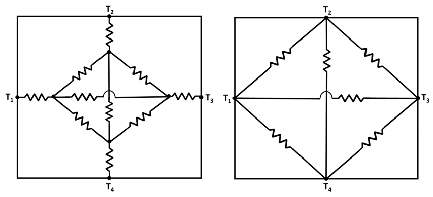
Oppenheim introduces radiosity nodes connected to surfaces through conductances that depend on emissivity, representing surface resistance to radiation heat transfer. These nodes are also interconnected via conductances based on geometric view factors. While Oppenheim’s radiation matrices are compact and efficient for solving large radiation models, computing direct radiative heat exchange for reduced models is more complex and less efficient than with the Gebhardt method.
The Gebhardt network calculates direct radiative couplings by accounting for all possible reflections through other surfaces. Although rarely used due to its larger matrices and increased runtime, it simplifies RTM generation by directly providing the equivalent radiative conductances needed for the TMM.
- Define the FILES MODLCF, VUFF, MODLF IN ASCII advanced parameter in the Advanced Controls simulation object to convert the output files to the ASCII format.
- Define the RADIATIVE CONDUCTANCE METHOD advanced parameter, where method is set to Gebhardt.
- Select the Element Center Method as Element Discretization in the Solver Parameters dialog box to reduce the nodes in the conductance network. It facilitates the extraction of the conductive couplings between the reduced zones.
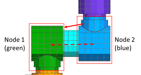
- Locate the MODLCF file that contains all the thermal couplings, capacitances
and heat loads for the thermal nodes, as well as additional data that will
not be needed for the RTM after the simulation is completed. To keep the
MODLCF file more manageable, it is best to deactivate any elements that will
not be included in the RTM before running the solution. The following is the
example of the MODLF file.

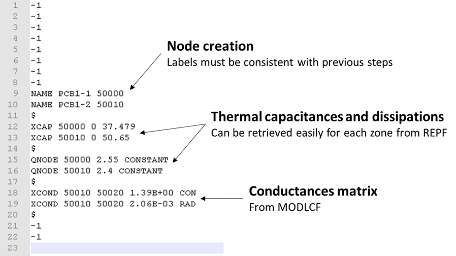
- Gather the required information from the runtime files and reformat in the
INPF format. The following is an example of a reformatted file.
Generating the geometrical mathematical model
- Delete all the internal mesh elements. They will be replaced by the TMM.
- Remove capacitance and thermal conductivity on the mesh elements in the GMM,
since they are included in the TMM to avoid accounting for them twice. You
can either:
- Set the mesh collectors as null shells.
- Apply override sets to the entire model and specify thermal conductivity and specific heat as 0.
- Simplify the mesh of each zone to reduce element count. If the meshes are CAD-associated, re-mesh them with a coarser resolution. To maintain equivalent heat inputs and outputs, the area and orientation should remain as similar as possible between the full and reduced geometry.
- Merge the remaining external mesh elements into zones as initially defined to create the link between the GMM and TMM using Merge Sets ensuring the ID matches the one used in the TMM. When the solver input file is written, the solver recognizes that this label is shared between the GMM and TMM and merges the nodes.
- Add the previously generated TMM as an include file in the solution parameters. Retain only the relevant data such as thermal node definitions, capacitances, dissipations, and the conductance matrix. Once this is done, the RTM is complete.
Recreating the TMM in Simcenter 3D using 0D elements and thermal couplings
- Lump the created zones, by removing 3D, 2D, and 1D elements, and replacing them with 0D elements.
- Specify the equivalent capacitance of each zone from the INPF.reduced file for 0D elements.
- Reapply all the boundary conditions, such as heat loads and thermal
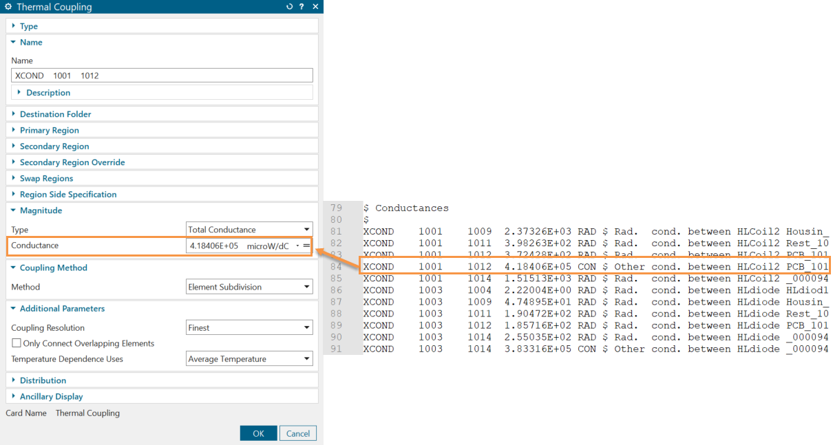
couplings, as specified in the INPF.reduced file.The following example demonstrates the conductive conductance between groups 1001 and 1012, sourced from the INPF.reduced file and applied in the thermal coupling.
