How to perform the HEEDS-based model update shapes solution process?

Introduction

The model update solution process uses the HEEDS solver, which does not require sensitivity data, offering compatibility with a broader range of design variables, solvers, and solution types compared to the SOL 200 Model Update based on Nastran SOL200 which is limited to only Nastran modal analysis.

The model update solution process optimizes the parameters in your model to match static, mode, or operational shapes results between a work and reference solution. It can update a wider range of solution and parameters.

The model update shapes solution process automatically generates objectives from error matrix plots, streamlining the process. Furthermore, constraints can be considered during optimization, ensuring that the updated model meets all necessary requirements.

Model update shapes solution process workflow

The following diagram summarizes the overall process for creating a model update shapes solution process.

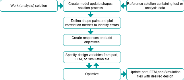
Use the following steps to perform the model update shapes solution process.

1. Create and solve a work solution, which represents the analysis model you would like to update.
2. Import the reference results by importing a test or analysis data.
   • Use the Test Reference command with the Structural Modal Test analysis type for a reference solution containing static, modal, or operational test data
   • Use the Analysis Reference command for the analysis reference results.
3. Create a model update shapes solution process using the Shapes command.
   • Select a reference solution.
   • Select a work solution.
   • Select a measurement type, for example Displacement, so the solver extracts displacement measures from the selected subcases.

   The model update shapes solution process automatically generates the node map, shape sensor sets, if the reference data is from test, and pairs work and reference shapes.

4. Review the model update shapes solution process.
   • Use mapping methods and filters to reduce the node map down to the nodes that you want to compare if your reference solution is from analysis.
   • Clone the initial sensor set and activate or deactivate sensor DOFs that are used to compute correlation metrics, if the reference data is from test.
   • View the shape pairs using side-by-side display and animations.
   • Plot correlation metrics to identify errors.
5. Create responses to monitor the impact of variables on your objectives and constraints. You can:
   • Right-click the selected pairs in the Correlation Details View and choose Create Response.
   • Right-click the selected cell or a group of cells in an error matrix and choose Create Response.
   In the Create Response dialog box:

   • Select the creation mode, for example, Combine to minimize the number of responses to track.
   • Select the type of response to create, such as MAC, X-Ortho, off-diagonal, or frequency.
6. Create objectives by selecting the Response node in the Simulation Navigator, right-clicking the selected responses in the Correlation Details View, and choosing Add to Objective.

   Specify whether the software:

   • Minimizes or maximizes the objective value to reach the minimum or maximum acceptable value of the response.
   • Minimizes the difference between the response value and a target value that you specify.
7. Set optional constraint specifications for the mass, volume, or weight of the model by right-clicking the Constraint node and choosing Create Constraint.

   The software uses the constraints values to determine the feasibility of the designs.

8. Create design variables using expressions and parameters from part, assembly FEM, FEM or Simulation files by using the Design Variables command. The optimizer varies the design variable values at each iteration to optimize the objectives.
9. Specify the optimization options, such as the number of evaluations, using the Option command and run the optimization using the Optimize command to let the software find the best design.

   When you run an optimization, the software completes the specified number of iterations, changing values for the design variable for each iteration and calculating the resulting values of the responses and objectives.

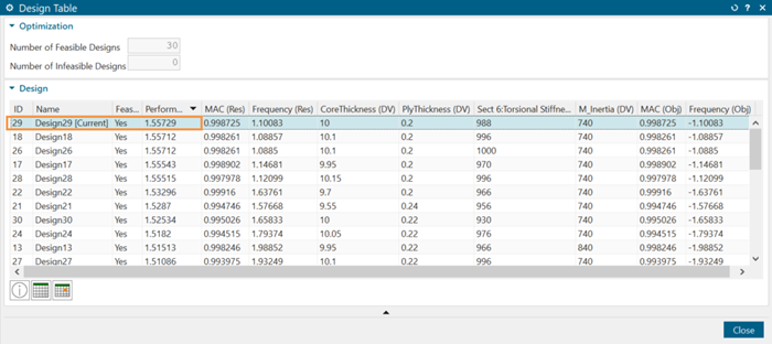
10. Examine the optimization results in the design table and select a current design with the highest performance rating.

    
    

    

    
    

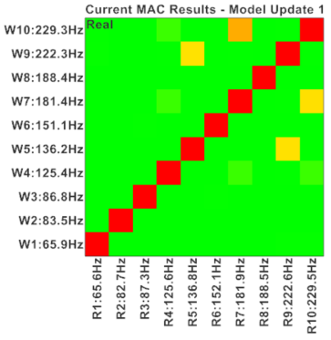
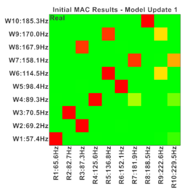
11. Plot the initial and current metrics.
    • Plot the MAC matrix before and after optimization by right-clicking the Shape Correlation Metrics node and selecting Plot MAC→Both to compare initial and current errors.
    • Display or animate the work shapes before and after optimization using the Plot Shapes command.
    • Plot the frequency of reference and work shapes by right-clicking the Shape Correlation Metrics node and selecting Plot Error Matrix.

      
      

      

      
      

12. Update the expressions and parameters associated to the part, FEM, assembly FEM and Simulation files with the current values of the design variables, which correspond to those of the selected design using the Update command.
13. Validate that the initial values of the design variables, the associated expressions and parameters have been updated.

Download the following example.zip, which provides the part files and step-by-step procedure.