Solution setup check
This topic explains how to validate initial conditions, transient-solution settings, memory usage, automatic time stepping, and overall model readiness before running the thermal solver.
This lesson may include hands-on exercises. Review the Discussion section for background information or click the button to proceed to the practical section.
Discussion
- Defining initial conditions
- Check the global ambient and initial conditions in the
Solution dialog box.
Define local initial conditions using the Initial Conditions constraint. Local conditions override global conditions.
- Configuring transient solutions
- Verify the following transient solution settings:
- Start and end time.
- Integration method.
Implicit is the recommended method.
- Time-step size.
Ensure that the time step isn't too large. A sensitivity analysis can be run on this if time permits.
- Convergence criteria.
To improve solve performance:
- Increase the maximum temperature difference convergence criterion.
- Use the implicit time integration method.
- Increase the integration time step.
- Memory optimization
- Verify that the machine is not running out of memory during the
solve.
Check the <simulation/model name>-<solution/analysis name>_verbose.log file for warnings related to the conjugate-gradient solver.
You can also request timing and memory information from supported thermal-solver modules using the following advanced parameters:
- INCLUDE TIMING INFO IN VERBOSE OUTPUT
- INCLUDE MEMORY INFO IN VERBOSE OUTPUT
- Using automatic time step
- Automatic time stepping can significantly improve transient-solution
efficiency.
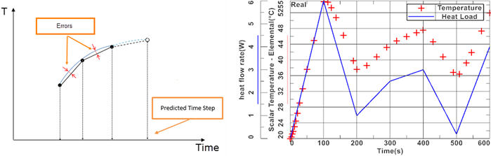
The automatic time step size calculation is based on the estimated error between a quadratic fit and a linear fit through three consecutively computed temperature values for two consecutive time steps.
As shown in the graph, the adaptive time stepping scheme creates smaller time steps around the times when the abrupt changes occur. The blue curve represents the time-varying heat load that is applied to a boundary condition, and each red dot represents the temperature value at the point where the boundary condition is applied. The dots that are close to each other indicate that the time steps are smaller at those times, to better capture the changes in the heat load.
- Running a model setup check
- Run a model setup check for the solution by:
- Right-clicking Solution and selecting Model Setup Check.
- Selecting the Model Setup Check check box in the Solve dialog box.
Review all reported warnings and errors before solving.
The Model Setup Check reports issues related to:
- Assembly FEM label conflicts.
- Simulation label conflicts.
- Mesh, materials, and physical properties.
- Groups.
- Loads, constraints, boundary conditions, such as invalid selections and values.
- Solutions.
Hands-on material
To gain experience with the topics discussed here, complete the following: