Post-processing and result validation
This topic explains how to verify thermal connections, boundary-condition behavior, fluid-network performance, and solver stability after the analysis completes.
This lesson may include hands-on exercises. Review the Discussion section for background information or click the button to proceed to the practical section.
Discussion
After the analysis completes, review the results to confirm that the thermal model behaves as expected. Post-processing helps you verify thermal connections, boundary-condition behavior, fluid-network performance, and solver stability.
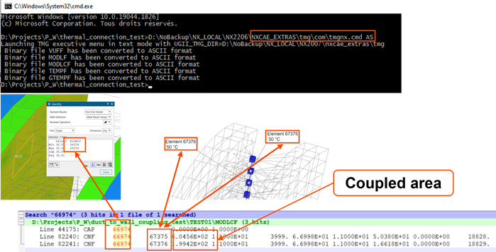
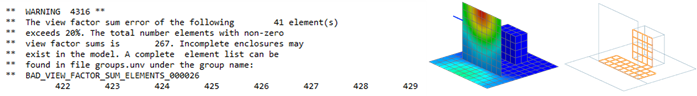
- Inspecting coupling areas per element in scratch files
- Inspect elemental coupling areas by converting the MODLCF file to ASCII
format either by:
- Using the executive menu command.
- Specifying a FILES MODLCF, VUFF, MODLF IN ASCII advanced parameter.
In the MODLCF file below, notice that the surface element 66974 is connected to elements 67375 and 67376.
- Verifying thermal connections
- Use the Thermal Connection result sets to verify that
primary and secondary elements are correctly connected thermally.
These result sets allow you to:
- Contour thermal connections.
- Inspect connected regions.
- Verify thermal continuity between components.
- Using the plot BC summary
- Include the PLOT BC SUMMARY advanced parameter to generate the
<simulation name>-<solution name>_data.html
file when using releases prior to 2606. Starting with the 2606 release, the
thermal solver generates this file by default. The thermal solver generates
the <simulation name>-<solution name>data.html
file where you can inspect various result quantities associated to boundary
conditions, thermal couplings, and named points.
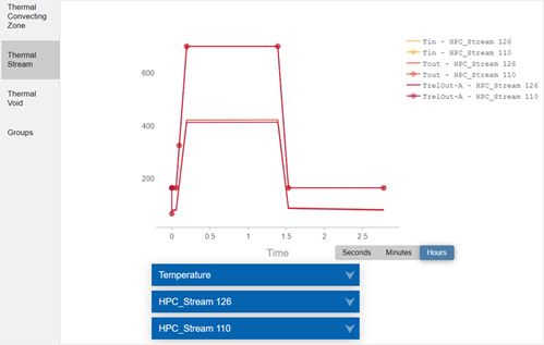
The graph below shows two stream inlet and outlet temperatures during a transient analysis. Convective Area can also be inspected in this report.
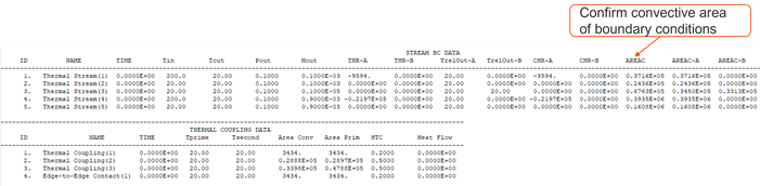
- Using BC summary tables
- Include the DISPLAY BC SUMMARY TABLES advanced parameter in the solution to
generate the <simulation name>-<solution
name>.bcdata file when using releases prior to 2606. Starting
with the 2606 release, the thermal solver generates this file by default.
The file stores the time and evaluated boundary condition data in the table
format. You can inspect various quantities related to thermal couplings,
voids, streams, and more. A common use case is to validate the convective
area.
- Displaying convective thickness and area factors
- In the Post Processing Navigator you can display:
- Convective Area Factor to visualize applied area factors on convective boundary conditions.
- Convective Thickness to visualize convective
areas associated with 2D element edges. The thermal solver computes
thickness differently depending on the 2D element type:
- For a 2D axisymmetric element, the element thickness is equal to 2π times the radius.
- For a 2D plane stress or strain element, the element thickness is equal to the specified thickness times the number of instances.
- For a 2D chocking element, the element thickness is equal to 2π times the radius minus the specified thickness times the number of instances.
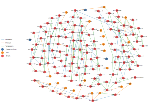
- Using the BC dependency graph
- When you include the BC DEPENDENCY GRAPH advanced parameter in the solution,
the thermal solver generates the
BCInterdependencyGraph.html file, that contains a
graph illustrating the dependencies, such as: temperature or mass flow,
between the thermal streams, voids, and convecting zones boundary conditions
in the solution. You can also display the dependencies, such as pressure,
swirl velocity, heat load, area correction, and heat transfer coefficient,
or choose only to display the temperature or the mass flow rate
dependencies, separately.
- Checking fluid pressures on walls from the thermal solve
- Pressure-definition errors are easy to overlook and can produce significant
deflection errors in coupled thermal-structural analyses.
Perform spot checks of pressure results at multiple time points to verify that wall pressures are physically correct.
- Running the model adiabatically
- Run the model adiabatically (HTC=0) and compare the results with
secondary-air-system predictions to confirm that windage-related heat pickup
is reasonable. Verify this by examining the 1D Fluid
Temperature, Total Absolute, or
Relative Fluid Temperature.
This comparison is valid only for adiabatic secondary-air models.
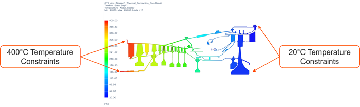
- Running a conduction only simulation
- Remove all convective and radiative boundary conditions and loads, but
retain thermal contacts and joints in the model.
Apply temperature constraints at both ends of the model. This allows you to confirm that thermal contacts are correctly modeled and serves as a check for specific heat in transient runs.
- Checking mass flow and stream nominal directions
- You can display:
- Mass Flow Vector to confirm mass flow directions within the fluid network. Use the Arrows command to view the direction of the mass flow in ducts and streams.
- Stream Nominal/Reverse Direction to contour and identify flow reversals: nominal (1) or reverse (-1).
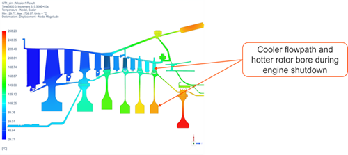
- Checking temperature gradients at shutdown conditions
- Temperature scaling issues are common in transient analysis. Inspect
shutdown temperature distributions to verify physically realistic transient
behavior.
- Thermal solver troubleshooting
- The following resources help troubleshoot thermal models:
- Review the following files: .log, verbose.log, and report.log.
- Inspect the partial .bun file.
- Apply the traceback patch.
- Simplify the model by removing some features.
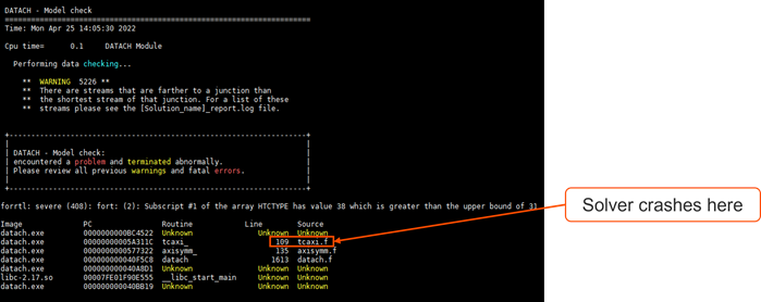
- Inspecting a log file
- The <simulation/model name>-<analysis name>.log
file is the primary troubleshooting file after a solver crash.
This log file may contain some specific details on why the model crashed such as:
- Warnings and error messages.
- Convergence data.
- Heat flow summary for steady state analyses.
- Inspecting a verbose file
- The <simulation/model name>-<analysis
name>_verbose.log file contains:
- Crash information.
- Timing statistics.
- Memory usage.
- Post-processing details.
- Solver execution details.
This log file may contain specific details about the cause of the crash and the process being executed at the time.
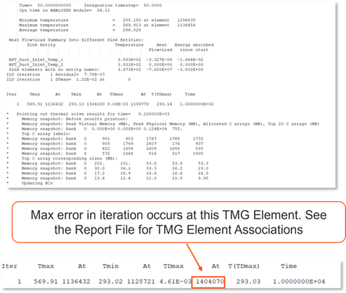
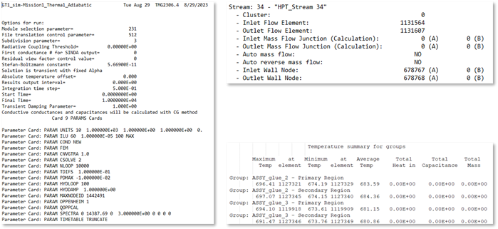
- Inspecting a report file
- The <simulation/model name>-<analysis
name>_report.log file contains calculation details, model
parameters, stream details, thermal solver created elements, results summary
of groups. Inspect the file to troubleshoot stream junction
interdependencies and to review elements created by the thermal
solver.
- Inspecting partial .bun file
- During a crash, a partial .bun file may be available.
Check the simulation directory for the available .bun file. If not automatically connected to the solution, import the .bun file into post-processing.
- Resolving warnings
- Review the messages in the Solution Monitor or the
log file for the thermal and flow solvers.
Import the solution warning groups and observe the failed elements by choosing File → Import → Simulation, select Simcenter 3D Thermal/Flow.
- Applying a traceback patch
- Applying a traceback patch requires referencing a new set of thermal solver
files before solving. The log file provides detailed information after a
fatal crash, including the code location and the line number where the crash
occurred.
You can request a traceback TMG patch, if it is not included.
- Simplifying the model
- Simplify the model to identify the issue if there is no clear cause for the crash. Clone the problematic solution and remove boundary conditions in sections. For large models, use Deactivation Set Advanced to deactivate meshes and reduce time steps to shorten solve time.
- Thermal mapping troubleshooting
- It is recommended to use the Simcenter3D Thermal/Flow
mapping solution.
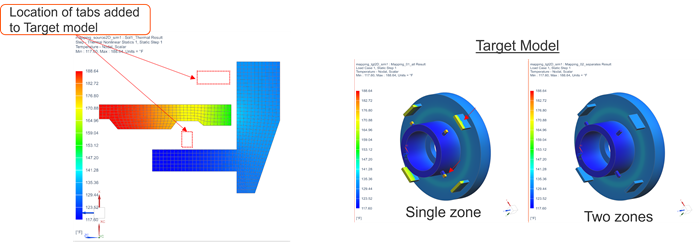
Common mapping issues include:
- Missing Association Zones when trying to set the Target Zones.
- Unexpected temperature gradients.
- FATAL 15018 – Target Zone <xxx> intersects target zone <yyy>.
Confirm that the source thermal model includes the Association Zones:
- Check for constraints in the source solution.
- Check the source .map or .xml file for constraints.
A map file size of ~32 kB likely indicates that no zones were defined.
- Confirm the target zone type matches the assigned source Association Zones.
- Confirm that the referenced .bun is the correct model.
Note:If the only change to the source model is the addition of Association Zones, the source .xml and .map files can be regenerated without re-solving the solution. - Resolving unexpected temperature gradients
- Use association and target zones to guide the mapping solver. If not
specified, the solver maps using the nearest source temperature based on
proximity. Ensure the source model's association zones cover the desired
regions and verify alignment with the correct 2D Solid
Option defined, if applicable.
- Resolving FATAL 15018 issue
- Mapping target zones cannot overlap. The solver will issue the FATAL 15018 error if they overlap. In the Target Zone, use Destination Nodes and exclude the face with shared nodes.
Hands-on material
To gain experience with the topics discussed here, complete the following: