Modify and solve a solution
Practice modifying solution parameters and solving a communications satellite thermal analysis.
Open the Simulation file
Open the model Simulation file and reset the dialog box settings.
- Choose File→Open and open communications_sat\communications_satellite_sim1.sim.
-
Choose File→Preferences→User Interface and on the Dialog and Precision page, reset the dialog box memory.
The model contains a transient solution with many results samplings to facilitate going over all the steps in this activity. Using these many sampling points is not standard practice.
Modify a solution
Modify a solution that contains predefined orbital heating and radiation simulation objects.
- In the Simulation Navigator, right-click the Transient node and choose Edit.
- In the Solve Options group, from the Run Directory list, select Simulation-Solution Name to generate a subdirectory in the working directory named with the current simulation and active solution.
- In the Solution Type group, select Transient from the Solution Type list.
- Click OK.
- In the Simulation Navigator, right-click the Transient node and choose Edit Solver Parameters.
-
On the Thermal Solver tab, in the
Transient Convergence Control group, type
0.01 Δ°C in the Maximum Temperature
Change box to set the value for the maximum temperature
change of any element between two consecutive iterations at each time
step.
When the temperature change of all elements between two consecutive iterations is below the specified value, the transient solution goes to the next time step.
- In the Conjugate Gradient Solver group, notice that in the Convergence Norm list, the MAX type of norm is used to calculate the convergence residuals for temperatures during the linear solve.
-
In the Convergence Criterion box, type
1e-07.
The Convergence Criterion tells the conjugate gradient solver when converged results are achieved. The lower the value of convergence criterion will result in a more precise solution.
- Click OK.
Explore the model
Explore the groups and boundary conditions in the transient solution.
-
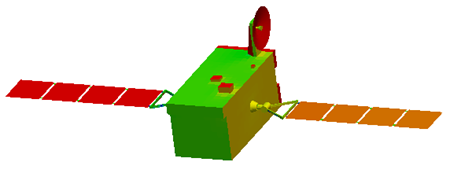
In the Simulation Navigator, expand the Groups node and click the 2 - Solar Panels node.
It highlights the solar panels elements as a group, on which you will display the group temperature results during the solve.
- Expand the Transient→Simulation Objects nodes and explore the existing boundary conditions.
Check the completeness of your model
Verify the model setup and resolve label conflicts.
- Choose Menu→Analysis→Finite Element Model Check→Model Setup.
-
Click OK in both dialog boxes.
The Information window displays label conflicts in the simulation.
-
In the Simulation Navigator, right-click the
communications_satellite_sim1.sim node and select
Simulation Label Manager to resolve the label
conflicts.
In the Labels group, on the Modeling Objects tab, observe that the Status is set to Conflict
 .
. -
In the Automatic Label Resolution group, click
Automatically Resolve
 .
.
- Click OK.
Start the solving process
Begin solving the transient solution and monitor its progress.
- In the Simulation Navigator, right-click the Transient node and choose Solve.
-
Click OK.
The Analysis Job Monitor dialog, Information window, and Solution Monitor open showing solving information.
- If the solve ends while still going through steps, click Yes in the Review Results dialog to keep monitor windows open.
Inspect the Solution Monitor
Review solving information and details in the Solution Monitor window.
- In the Solution Monitor, click Inspect to lock the running message display and scroll through details.
-
Notice the following:
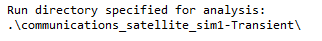
- At the beginning, you can see the run directory you specified in the
previous section:
- Under Model Summary, you can see the number
of nodes and elements used in the thermal model:

- At the beginning, you can see the run directory you specified in the
previous section:
- Scroll to explore the other information in the Solution Monitor window.
- Click Inspect to cancel the lock.
Monitor the real-time results in the Solution Control Monitor
Monitor real-time temperature distribution during the transient solution.
-
In the Solution Monitor, click SC Monitor
 to open the Solution Control
Monitor.
The model mesh displays when it becomes available by the solver. For a thermal analysis, this is when THERMAL – Thermal Analysis is displayed at the bottom of the Solution Monitor.
to open the Solution Control
Monitor.
The model mesh displays when it becomes available by the solver. For a thermal analysis, this is when THERMAL – Thermal Analysis is displayed at the bottom of the Solution Monitor. -
In the Results group, from the Results
Type list, select Temperature [C] to
display the temperature distribution at each time step.
The temperature results evolves during the transient solution. - In the Results group, click Group.
- In the Thermal-Elemental group, make sure that the Solar panels check box is selected.
-
Click Apply.

The software displays the elemental temperature distribution only on the solar panels elements group.
Display convergence graphs
View convergence graphs for current step, iterations, and full model.
-
In the Solution Monitor, choose Graphs
 →Convergence→Current Step.
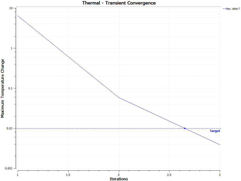
Notice the target maximum temperature change, which you specified in the previous section. -
Choose Graphs→Convergence→Iterations.

It displays the number of iterations at each time step for the thermal solver to converge. -
Choose Graphs→Track Results→Full Model.
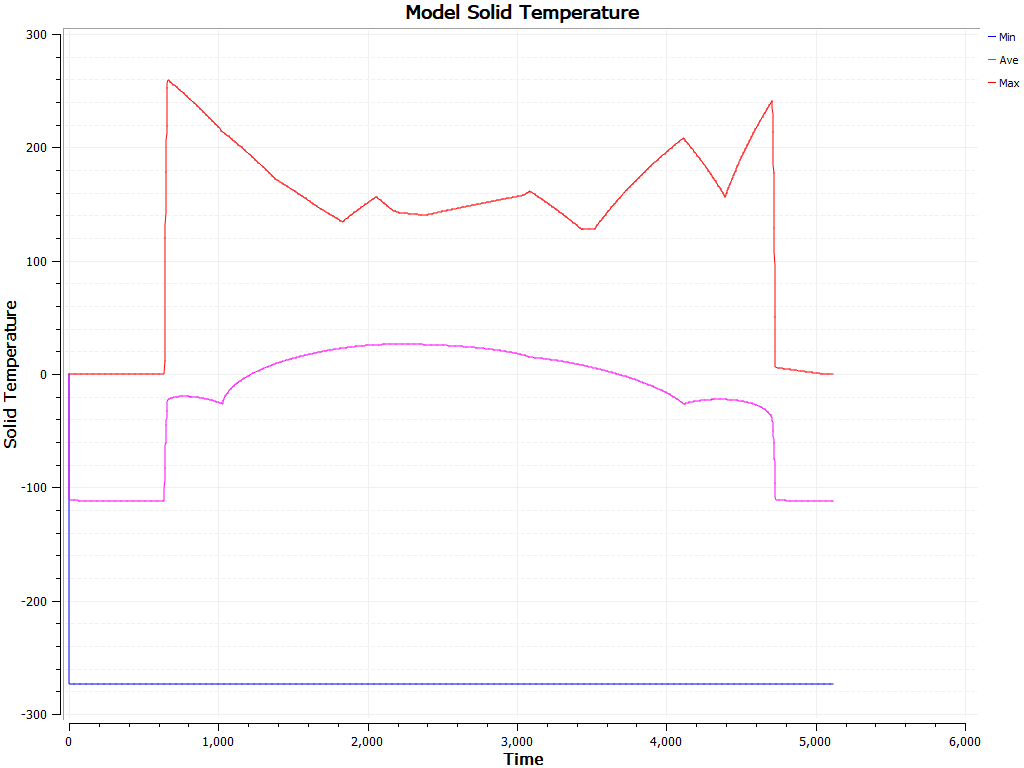
It displays the minimum, average, and maximum values of solid temperatures.
Abort a solution
Abort the transient solution and close monitoring windows.
- In the Solution Monitor, click Abort.
-
In the Abort Solution dialog, click
Yes.
The Solution Monitor, Solution Control Monitor, and all graphs are closed.
- Close the Information window.
- In the Analysis Job Monitor dialog, click Cancel.
- In the Simulation Navigator, right-click the Transient node and choose Browse.
-
Open the communications_satellite_sim1-Transient
folder and double-click the
Solution_Monitor_Graphs.html file to view convergence
graphs.
The software creates a copy of convergence graphs in the html format.
- Hover over any graph to use the post processing tools.