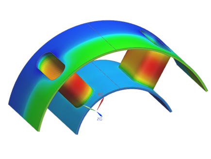
Map convective results
Learn how to extract fluid temperature and heat transfer coefficient (HTC) results from a 2D Whole Engine Model and map them to a 3D submodel.
Introduction
In this tutorial you will:
- Map fluid temperature and heat transfer coefficient (HTC) from 2D to 3D.
- Create Result Probe to extract HTC on face.
- Create Field from Results.
- Apply fields on 3D cyclic geometry.
Load the 2D model and inspect thermal boundary conditions
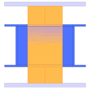
Review applied streams, convective zones, and overlapping boundary conditions prior to extracting results.
- Choose File→Open and open convective_results/2D/strut_sim1.sim.
- Inspect applied thermal streams in the ST folder and thermal convective zones in the CZ folder.
- Observe that the CZ2_FACE and ST10 boundary conditions overlap on the same face.
- Confirm that CZ2_FACE uses an HTC of 300 W/m²K, when SCALER=1, and ST10 side A uses an HTC of 15 W/m²K, when SCALER=1.
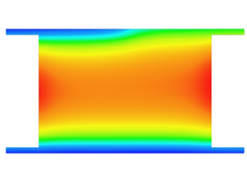
Solve the 2D model and inspect convection results
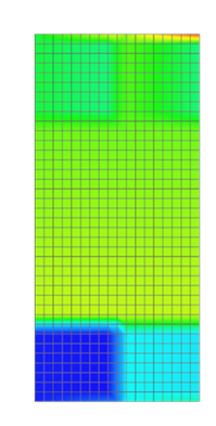
Solve the transient 2D model and evaluate convection coefficient results, including behavior at regions with overlapping boundary conditions.
-
Use the Identify Results command to inspect the
temperature on the 4391 element.
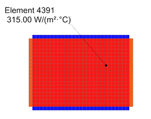
Verify that the value is 315 W/m²K, which represents the sum of the heat transfer coefficients from the overlapping boundary conditions. Understanding this behavior is important, as it limits what data can be directly mapped to the 3D thermal model. For this region, the boundary conditions will be handled differently in the 3D model. -
Under Post View, display solver-created 1D elements
to observe available convective results on edges.
Create result probe to extract HTC from a face
Create a result variable and probe to extract convection coefficient data from strut faces for mapping to the 3D model. The Result Probes command provides an automated method for extracting result fields from the analysis. Because the 3D model contains repeating cyclic sectors, an axisymmetric field will be used to ensure the mapped results are applied consistently across all sectors.
-
Choose
 to create result variables with
the following settings:
to create result variables with
the following settings:
- Name = HTC
- Result Type = Convection Coefficient
- Coordinate System = Absolute Rectangular
-
Choose
 to create result probes on the faces of the
strut referencing the HTC variable. Set the following settings:
to create result probes on the faces of the
strut referencing the HTC variable. Set the following settings:
- Name = HTC_STRUT_FACE
- Formula = HTC
- Load Case = Ignore
- Selection Type =
Faces
- Result Type = Convection Coefficient
- Unit = W/m2°C
- Output Options = Field
- Independent Domain = 3-D
- Time, Axisymmetric Plane
- Select the Create Output check box to automatically generate a field from the result probe
Verify that a corresponding field appears under Fields in the Simulation Navigator.
Create a field from results to extract fluid temperature on face
Extract the fluid temperature in post-processing by creating a field from the displayed results. Use this method when you cannot extract certain quantities—such as Total Absolute Fluid Temperature at the wall—with result probes.
-
Use the Identify Results command and select all
displayed elements using the Box(All) selection
method.
-
In the Identify dialog box, click Create
Field
 to create a field from results with the
following settings:
to create a field from results with the
following settings:
- Name = FLT_STRUT_FACE_Manual
- Independent Domain = Time, Axisymmetric Plane
- Dependent Domain = Temperature
- Duplicate Values = Average
Create field from results for HTC and fluid temperature for 1D elements
Export all of the results into one field to make the import and export of fields more manageable.
-
Click Create Field
to create a field from results with the
following settings:
- Name = ALL_1D_FLT
- Independent Domain = Time, Axisymmetric Plane
- Dependent Domain = Temperature
- Duplicate Values = Average
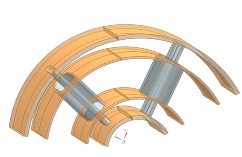
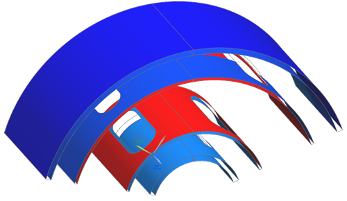
Load the 3D model and inspect thermal boundary conditions
Open the 3D submodel and review existing convection boundary conditions.
Import fields and modify convection definition
Import fields generated from the 2D model and assign mapped fluid temperature data to existing 3D convection boundary conditions.
-
In the Temperature Value box, click
 and choose Select Existing
Field and select the existing field you imported
representing fluid temperature on the strut face.
and choose Select Existing
Field and select the existing field you imported
representing fluid temperature on the strut face.
-
Set Time to 700s and click
Plot
 .
.
Use the Feature
 command in the
Display tab to show only feature edges in the
postview.
command in the
Display tab to show only feature edges in the
postview.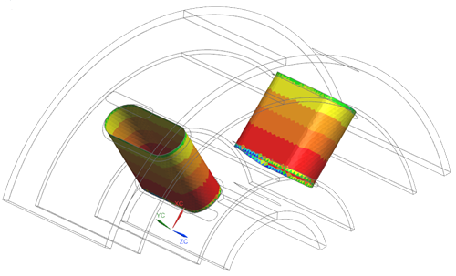
Create convection boundary condition on strut
Apply mapped convection boundary conditions to strut faces using imported HTC and fluid temperature fields.
-
Choose

-
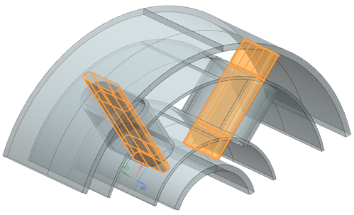
Select strut faces using the Tangent Faces method as
shown.
-
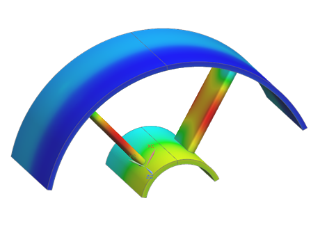
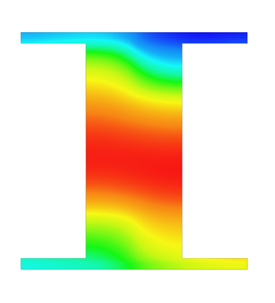
Plot contours at 700[s] to verify axisymmetric field behavior.
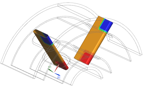

Convection Coefficient Temperature Value
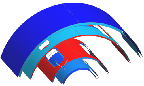
Apply convection to surfaces corresponding to 1D elements
Apply convection boundary conditions on 3D surfaces corresponding to 1D edge locations from the 2D analysis.
-
Select the faces as shown below.
24 faces are selected. These faces correspond to the locations of 1D elements in the 2D analysis. We can include all surfaces in one convection to environment constraint to save time.
-
Plot contours at 700[s] to confirm correct application.
Convection Coefficient Temperature Value
Solve 3D model and compare with 2D results
Solve the 3D model and compare metal temperatures to validate the mapped convection results.
-
Verify consistency of mapped convective behavior.
Additional notes
- Mapping HTC and fluid temperature allows asymmetric effects to be introduced in 3D submodels.
- When applying known fluid temperatures and heat transfer coefficients, either a Thermal Convecting Zone or a Convection to Environment can be used. However, if total temperature effects must be considered, a Thermal Convecting Zone is required.
- If only metal temperatures are required, use the separate Thermal Mapping workflow instead.