Extract and calculate tip clearance

Learn how to extract displacement data and contact gap results to calculate blade tip and flowpath clearances.

Introduction

One of the primary objectives of a whole engine model is to predict clearances throughout the engine, including blade tips, labyrinth seals, rim cavities, and axial gaps in the flowpath. Accurate clearance prediction leads to improved performance estimates and greater engine reliability.

Gas turbine design teams frequently optimize clearances through sensitivity studies, varying parameters such as geometry, materials, cooling network configurations, and transient operating conditions.

In this tutorial, you will:

Create result probes at defined points.
Compare Cartesian and cylindrical displacements.
Extract gap distance from contact results.
Manually extract displacement data.
Calculate clearances, including the effect of angled blade tips.

Load the thermal plugin

Enable the ExpressionsPlugin.dll if not already active. The predefined boundary conditions in the model use heat transfer coefficient (HTC) correlations implemented through custom expressions. These correlations require the plugin to evaluate correctly during the simulation.

Choose File > Utilities > Customer Defaults.
Click Simulation, expand Pre/Post, and scroll to Expressions.
On the Plugin tab, select the Use Custom Plugin check box and in Custom Plugin, type the full path to the ExpressionsPlugin.dll file, as plugin\ExpressionsPlugin.dll.
Click OK, exit Simcenter 3D, and restart the application to activate the plugin.

Define assembly load options

Configure search folders to load the workshop model.

On the Home tab, click Assembly Load Options .
From the Load list, select From Search Folders.
In the Add Folder to Search box, browse to the clearance folder.
Append \... to the end of the path so it appears as clearance\....
Adding \... allows the software to search the selected folder and all its subfolders. However, this option is not recommended for complex or deeply nested directory structures, as it may significantly increase search time.
Click Add to include the path in the search list.
Remove any existing paths that are no longer needed.
Click OK.

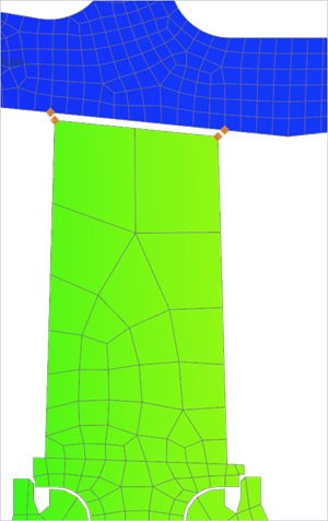
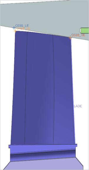
Inspect points and contact definitions

Review named points and inactive contact definitions used for clearance extraction.

Choose File→Open and open clearance\ASSY\GT1_sim.sim.
Press Ctrl and W, and next to Points click Show Points.
Choose File > Preferences > Visualization.
Under View, click Decorations, and set Show Object Names to Work View to display object names.
Observe the named points at the blade tip locations as shown.
Right-click a named point and select Properties.
On the General tab, observe that a name is assigned to the point in the Name box.
These named points will be used when extracting data using result probes.
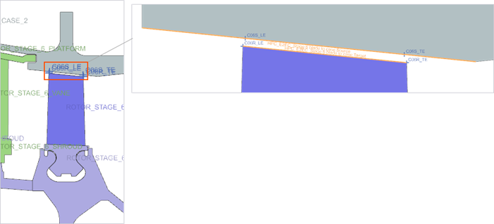
In the Simulation Navigator, under HPC_Blade_Tips, right-click HPC_E2EC_Stage 6 blade to case to inspect the edge to edge contact defined on the last stage of the compressor.
In the Local Contact Pair Parameters, click to inspect the Local Overrides contact parameters.
Within the contact parameter settings, observe that the Interface Behavior (INTRFC) is set to Inactive. An inactive joint allows the Nastran solver to compute and report gap distance results without affecting structural displacements or stresses. In this scenario, the contact is intentionally set to inactive so it can be used solely for post-processing clearance results, without influencing the solution.

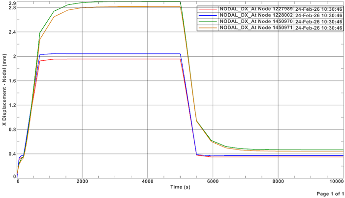
Manually graph and export displacement data

Plot displacement results and export data for comparison.

In the Simulation Navigator, expand Results and double-click Structural to load results.
The results data is available in the starting files.
Plot Displacement in the X direction.
Choose Results > Tools > Create Graph to create the across iterations graph on any of the compressor blade tips, for example stage 6.
In the X Axis group, from the Display list, select Time.
In the Graph Title box, type NODAL_DX.
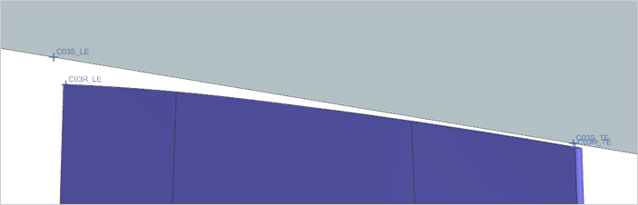
In the Y Axis group, from the Method list choose Pick from Model, and select leading and trailing edge nodes at a blade tip of stage 5 as shown.
Click OK and in the Viewport dialog box, click Create a New Window to Plot .
Click each curve in the graph, right-click the selection and choose Export to export the file to a CSV format.
Specify a path and filename.
This manual node-selection method is quick and requires no advanced setup. However, it is not easily repeatable between solves, and the data series names do not clearly indicate their physical locations. This makes subsequent post-processing more tedious, as node numbers must be manually tracked.
Choose Results > > Context > Return to Home .

Setup result variables and compare Cartesian and cylindrical displacement

Explore differences between Cartesian and cylindrical X displacement.

Choose Results > Manipulation > Result Probe to create result probes for cartesian X and for cylindrical X displacement.
In the Name box, type DX_3D_Tips.
In the Formula group, click Create Result Variable to create result variable for the Cartesian displacement.
In the Name box, type DX.
From the Result Type list, select Displacement.
From the Coordinate System list, select Absolute Rectangular.
Click OK.
From the Load Case list, select Ignore, and set the following:
- Iteration Category = None
- Iteration Selection = All
From the Selection Type list, choose Points and select the points on the leading edge and trailing edge of the stage 3 compressor blade, which are labeled C03R_LE and C03R_TE.
Create another Result Probe for cylindrical X displacement.
Set Name to DX_CYL_3D_Tips.
In the Formula group, click Create Result Variable to create result variable for the cylindrical displacement.
In the Name box, type DX_CYL.
From the Result Type list, select Displacement.
From the Coordinate System list, select Absolute Cylindrical.
Select the same points: C03R_LE and C03R_TE.
In the Simulation Navigator, under the Results Probe node, right-click each probe and select Create Graph.
Right-click the graph and select Probing Mode > Single X to compare the results.

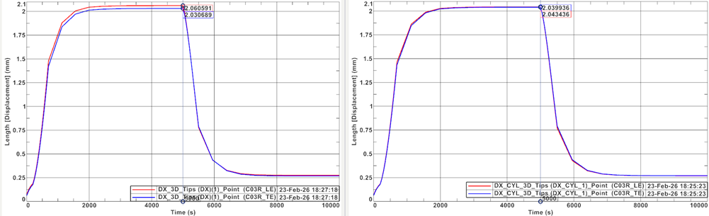
Because the blade is modeled in 3D, slight differences between Cartesian X and cylindrical X displacement are expected.
For rotating machinery, cylindrical X displacement should be used, as it represents true radial movement relative to the engine centerline.

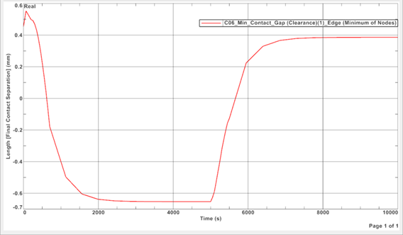
Setup result probe for final contact separation

Extract minimum blade tip clearance from contact results.

Create a result probe on the stage 6 blade tip using the following:
- Name = C06_Min_Contact_Gap
- For the Result Variable:
  - Name = clearance
  - Result Type = Final Contact Separation
  - Coordinate System = Absolute Rectangular
From the Load Case list, select Ignore and set Iteration Selection to All.
Form the Selection Types, choose Edges and select the shown edge as users are interested in the minimum clearance at the blade tip.
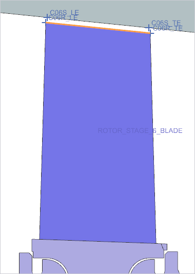
Select the Compute On Individual Geometry check box and from the Geometry Value, select Minimum result across the edge of the blade tip.
Create and review the graph.

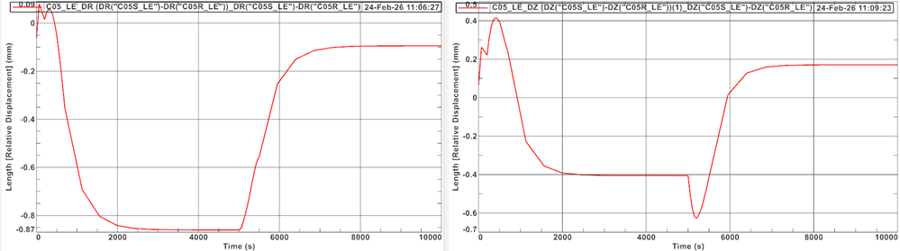
Setup result probe for delta displacement using built-in functions

Create a result probe using built-in functions to compute relative radial and axial displacement.

Create two result probes on the stage 5 leading edge to extract delta radial displacement and delta axial displacement, using the following settings:


Settings	Radial displacement	Delta axial displacement
Name	C05_LE_DR	C05_LE_DZ
Formula	DR("C05S_LE")-DR("C05R_LE")	DZ("C05S_LE")-DZ("C05R_LE")
Selection Type	None	None
Result Type	Relative Displacement	Relative Displacement

These result probes calculate relative movement between the rotor and stator points. If it is desired to also include the cold gap based on the initial position of points, the X() function can be used with the point names as an argument.

Graph and export results.

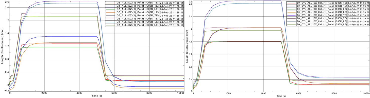
Setup result probe for radial and axial displacement of multiple points

Create a single probe to extract data for multiple blade locations.

Create a result probe on multiple points using the following settings:with formula DZ on points C03R_LE, C03S_LE, C03R_TE, C03S_TE, C05R_LE, C05S_LE, C05R_TE, and C05S_TE.
- Name = DZ_ALL
- Result Variable:
  - Name = DZ
  - Result Type = Displacement
  - Component = Z
  - Coordinate System = Absolute Rectangular
- Selection Type = Points
- Select 8 points at leading edge and trailing edge of compressor blades 3 and 5, labeled as: C03R_LE, C03S_LE, C03R_TE, C03S_TE, C05R_LE, C05R_TE, 05R_TE, and C05S_TE.
In the Simulation Navigator, right-click the DZ_ALL result probe and select Copy To > Baseline.
Edit the copied result probe, rename it to DX_CYL_ALL, and update the expression to DX_CYL.
Graph and export CSV files for further processing.

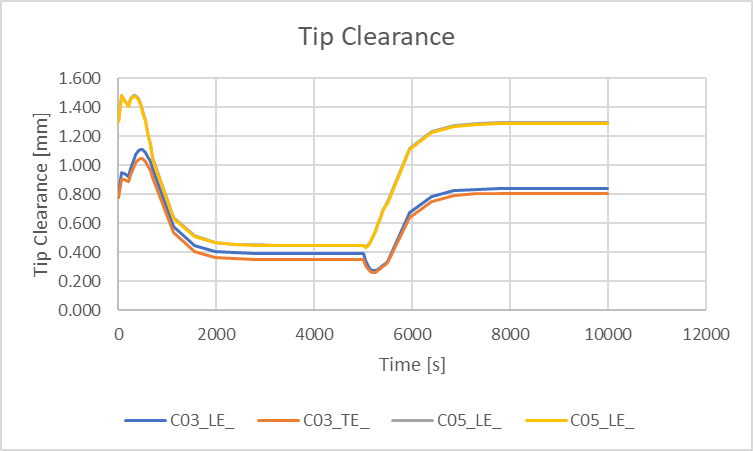
Calculate blade tip clearance

Compute conical blade tip clearance using radial and axial displacement components.

Compressor and turbine blade tips can be either conical or radial. With conical blade tips, both the axial and radial relative movements of rotor and stator will contribute to the tip clearance. The contribution of each displacement vector needs to be handled separately as shown:

Where:

DR is a displacement in radial direction.
DZ is a displacement in axial direction.
DTIP is a displacement perpendicular to blade tip.
Tip Angle is a blade tip angle relative to axis of rotation.

Open the clearance\GEO2\ASSY\Clearance_Post_Processing.xlsx excel spreadsheet, which includes exported data and calculations of blade tip clearances.
Inspect the Tip_Angles tab.
Observe the measurements of the conical blade tips, and the expressions used to calculate the axial and radial impact on tip clearance (columns AI and AJ).
Review DR and DZ tabs containing exported data from Simcenter 3D.
Inspect formulas in the Clearance_Calcs tab by clicking on the cell B2.
This cell is not only a lookup table, but also subtracts the displacement at time=0 from all of the values to ignore initial deflections in the engine. During assembly of the engine, there are some distortions based on clamping loads and gravity, and not all of those effects are accounted for in the 2D/3D WEM. The end goal of clearance analysis is to specify the cold build clearances required in the engine after assembly, and so these effects can often be ignored. Different design teams will most certainly have different design philosophies here.
Inspect cell F2.
Notice that columns B:E are axial and radial displacements of the rotor and stator at the leading edge. Column F calculates the relative movement between rotor and stator in the axial and radial direction, and applies the multiplier defined on the Tip_Angles tab.
Inspect the small table starting at W19.
The first column represents the minimum closure observed during the transient cycle. The assembly (cold build) clearances need to be at least this large, and typically there are some margins of safety applied, or other effects accounted for. The second column is the cold build clearance, which is based on the previous column and includes a 50% margin of safety. The last column is hot running clearances, which can be obtained by adding the relative displacement at time=5000[s] to the cold build clearance. This is the number that would be shared back to performance and aerodynamic teams.
Observe the graphs, which show the relative closure, as well as the tip clearance, during the transient cycle.

Additional notes

Consider additional 3D effects such as gravity, vibration, non-axisymmetric temperatures, and tolerance stackups.
Clearances are defined based on tolerance stackups of components and assemblies. Therefore, clearances are also defined with tolerances.
Axial clearances are more difficult to control, especially on the turbine side, because the displacement is based on the thermal growth and transient behavior of the whole engine.