Define radiative heating
Learn how to define a radiative heating source for a thermal analysis of a headlamp.
Open the model Simulation file
Open the Simulation file and reset the dialog box settings.
- Choose File→Open and open headlamp\lamp_fem1_sim1.sim.
- Choose File→Preferences→User Interface and on the Dialog and Precision page, reset the dialog box memory.
- Click OK.
Explore the model
Explore the predefined boundary conditions.
In the Simulation Navigator, explore the following
boundary conditions:
- The main enclosure radiation with the faces of the entities that make the internal cavity of the lamp.
- The convection of air around the head lamp with a constant convection coefficient of 5 W/m2C.
- The Thermal Void load that defines the fluid material, its heat load, and its capacitance in the internal cavity of the lamp.
Set thermo-optical properties
To save time, all thermo-optical modeling objects have been created and assigned to their proper mesh collectors. For the bulb and filament mesh collectors, define the thermo-optical properties.
- In the Simulation Navigator, double-click the lamp_fem1.fem node.
- Choose the Home tab → the Properties group → Modeling Objects.
-
In the Selection group, select
bulb, and click Edit
 .
.
- In the Infrared Properties group, in the Emissivity box, type 0.4.
- In the Solar Properties group, in the Absorptivity box, type 0.15, in the Transmissivity box, type 0.85.
- Set Index of Refraction to 1.4.
- Click OK.
-
Repeat the 3-7 steps to define the following thermo-optical properties for
the filament:
- Emissivity = 1 in the Infrared Properties group
- Absorptivity = 1 in the Solar Properties group
- Click Close.
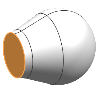
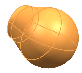
Define an enclosure for the bulb
Define radiation on the bulb of the lamp.
- In the Simulation Navigator, double-click the lamp_fem1_sim1.sim node.
- In the Simulation Navigator, expand the lamp_fem1.fem node → Polygon Ggeometry.
-
Next to the Plygon Geometry node, click
 and next to the
bulb node, click
and next to the
bulb node, click  to show the bulb only.
-
Choose Home tab → the Loads and
Conditions group → Simulation Object
Type list → Radiation
 .
.
- In the Name box, type Bulb enclosure.
-
In the Top Side Region, select the shown face.
-
In the Bottom Side Region, click Select
Object, and select the following six faces.
- In the Parameters group, clear the Include Radiative Environment check box and from the Element Subdivision list, select 1.
- Click OK.
-
In the Simulation Navigator, next to the
Simulation Object Container node, click .
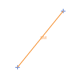
Define radiative heating parameters
Model the 13 W emitted by the resistor using a radiative heating boundary condition.
- In the Simulation Navigator, hide Polygon Geometry and show the 1D Collectors node to display the filament.
-
Choose Home tab → Loads and
Conditions group → Simulation Object
Type list → Radiative Heating
 .
.
- From the Type list, select Illuminate Selected Elements.
- In the Top Border bar, from the Filter list, select Element.
-
In the Top Side Emitting Region group, click
Select Object and select the shown element.
- In the Simulation Navigator, under Polygon Geometry, show the bulb node.
-
In the Top Side Illuminated Region group, click
Select Object and select the shown face.
-
In the Bottom Side Illuminated Region group, click
Select Object and select the shown 6 faces.
- In the Spectrum group, ensure Solar is selected.
- In the Magnitude group, in the Power Value, type 13 W.
- From the Element Subdivision list, select 1.
- Click OK.
-
In the Simulation Navigator, next to
Simulation Object Container, click .
Set the solver parameters
Enable result options.
- In the Simulation Navigator, right-click the Solution 1 node and select Edit.
- On the Results Options tab, under Radiative Source Fluxes, select Incident Fluxes, Transmitted Fluxes, and Reflected Fluxes to show the radiative flux that is received, transmitted, and reflected by the elements with transparent materials selected in the Radiative Heating simulation object coming from the source.
- Click OK.
Solve the model
- In the Simulation Navigator, right-click the Solution 1 node and choose Solve.
- Click OK.
- Wait for the solve to end, before proceeding. The solve takes around 10 minutes to complete.
- In the Review Results dialog box, click No.
- Close the Information window.
- In the Analysis Job Monitor dialog box, click Cancel.
Review the temperature results
- In the Simulation Navigator, expand the Solution 1 node, and double-click the Results node to load the results.
- In the Post Processing Navigator, expand the Thermal node, and double-click the Temperature - Nodal node.
- Expand the Post View 1 node → lamp_fem1.fem → 2D Elements
-
Click next to
cover_lens.
-
Choose Results tab → Display
group → Feature
 .
.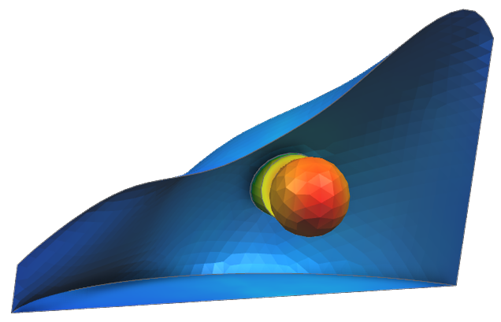
Observe the radiative flux results
- Choose Results tab → View Layout group → Four Views.
- Double-click the Absorbed Radiative Flux, Radiative heating – Region Emitting from Top Side – Elemental node to show the absorbed radiative flux results.
- Under the Post View 1 node → lamp_fem1.fem → 2D Elements, hide the bulb mesh.
- Right-click the Incident Radiative Flux, Radiative heating – Region Emitting from Top Side – Elemental, select New Plot and click the right view port.
- Under the Post View 2 node → lamp_fem1.fem → 2D Elements, hide the bulb and the cover_lens meshes.
- Right-click the Reflected Radiative Flux, Radiative heating – Region Emitting from Top Side – Elemental, select New Plot and click the left bottom view port.
- Under the Post View 3 node → lamp_fem1.fem → 2D Elements, hide the bulb and the cover_lens meshes..
- Right-click the Transmitted Radiative Flux, Radiative heating – Region Emitting from Top Side – Elemental, select New Plot and click the right bottom view port.
- Under the Post View 4 node → lamp_fem1.fem → 2D Elements, hide the bulb and the cover_lens meshes.
-
Choose Results tab → View
Layout group → Synchronize All Views
 .
.
- Click the first view port, press Ctrl, and select the other three view ports.
-
In the Top Border Bar, click Backface Culling
 .
.
-
Choose Results tab → Result
group → Top and Bottom
 to display results for both the top and bottom
of shell elements simultaneously.
When viewing top and bottom results at shell element recovery points, you must enable Backface Culling to render results on both sides of the element. For all other shell element result locations, Backface Culling displays only the top side, which helps you quickly identify whether the 2D element normals are consistent across the model.
to display results for both the top and bottom
of shell elements simultaneously.
When viewing top and bottom results at shell element recovery points, you must enable Backface Culling to render results on both sides of the element. For all other shell element result locations, Backface Culling displays only the top side, which helps you quickly identify whether the 2D element normals are consistent across the model. -
Choose Results tab → Display
group → Feature
.
-
Choose Results tab → Result
group → Average On/Off
 to set up nodal averaging across
all adjacent elements for elemental and element-nodal results for a smoother
display.
to set up nodal averaging across
all adjacent elements for elemental and element-nodal results for a smoother
display.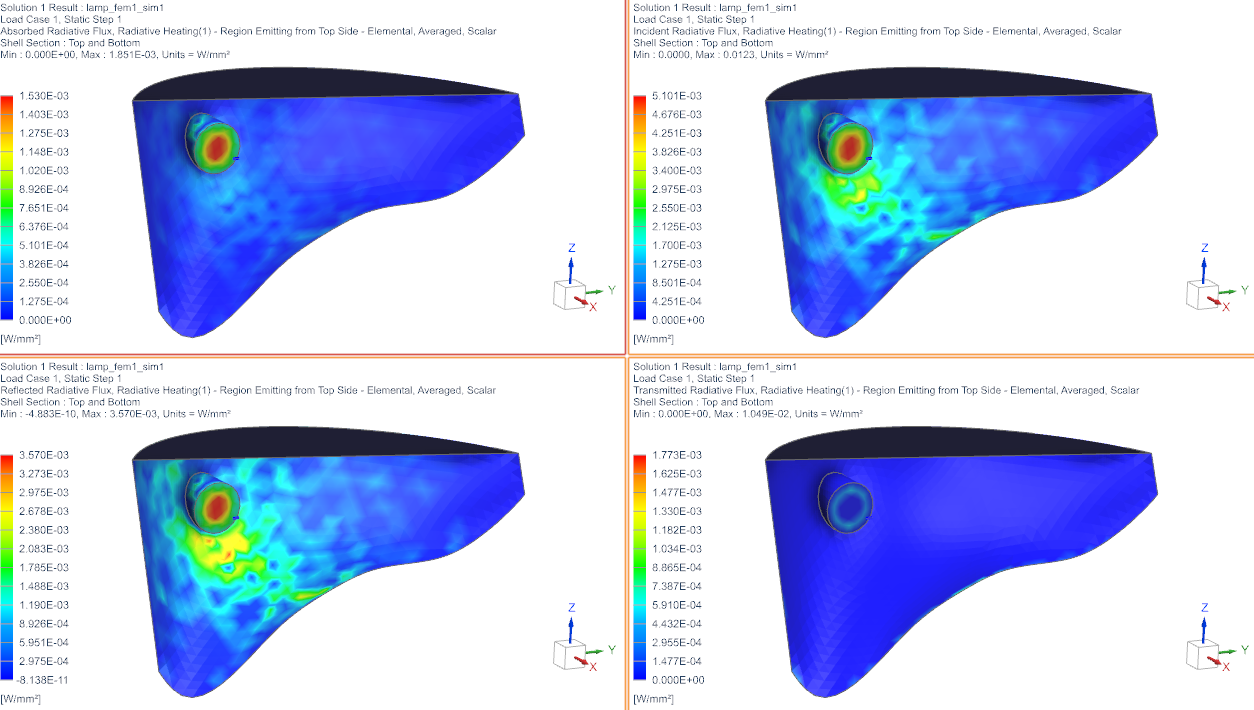
Observe that most of energy received by the reflector is being reflected back.