VVT41 - Heat transfer in a conical model with thermal void load conditions
| Test case |
|---|
| SVTEST282 |
Description
The purpose of this validation test is to determine the temperature distribution along the axial direction of a conical model with thermal void boundary conditions. The test evaluates the accuracy of simulation results by comparing them with analytical solutions under steady-state heat transfer conditions for a 3D model and corresponding 2D axisymmetric model.
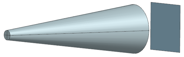
Geometry
The 3D model geometry consists of a truncated cone extending axially from 50 mm to 250 mm, with a taper ratio of a = 0.25. The base diameter at the smaller end is D1 = 12.5 mm, and the top diameter at the larger end is D2 = 62.5 mm. A 60 × 60 mm 2D plate is placed parallel to the larger end of the cone.
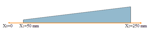
The corresponding 2D axisymmetric model is constructed using a trapezoidal profile on the YX plane, representing a cross-section of the cone, with the axis of rotation aligned along the X-axis.
Simulation model
A 3D mesh is generated using parabolic hexahedron elements that are 5 mm in size. The 2D plate is meshed using parabolic triangular elements, also that are 5 mm in size.
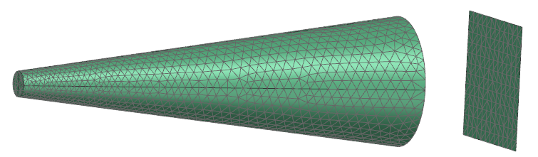
The 2D axisymmetric model is meshed with axisymmetric parabolic triangular elements of 5 mm in size.
The meshed elements have the following material and physical properties:
- Material for the cone and 2D plate: Aluminum_2014
- Mass density: ρ = 2794 kg/m3
- Thermal conductivity: k = 0.3 W/m·°C
- Environmental fluid material: Air
- Mass density: ρ = 1.2041 kg/m3
- Specific heat at constant pressure: Cp = 1004.5 J/kg·K
Boundary conditions applied on the solid 3D model and 2D axisymmetric cone:
- Temperature constraint applied on the smaller end of the cone of 200 °C.
- Temperature constraint applied on the larger end defined by a function of VT(1), referencing the thermal void temperature.
Boundary conditions applied to the plate:
- Temperature constraint of 600 °C.
- Thermal Void load with a head load of 10W applied to the plate surface, with a heat transfer coefficient of 10 W/ (m2·°C)
This model uses the Simcenter 3D Multiphysics solver.
The following solver options are set:
- Solver = Simcenter 3D Multiphysics
The following solution options are set:
- Solution Control: Element Discretization is set to Finite Element Method in the Thermal Solution Parameters modeling object.
Theory
The energy balance for a controlled volume for steady-state conditions is:
The fluid temperature at the boundary of the larger conical surface is:
where:
- Ts is the surface temperature of the cone.
- Tf is the fluid temperature at the boundary of the cone.
- Q is the added heat to the system.
- h is the heat transfer coefficient.
- A is the convection surface area.
The heat flux along the cone is:
Integrating the heat flux equation yields the temperature distribution along the X-axis:
where:
- k is the thermal conductivity of the material.
- a is a taper ration of cone.
- x is the axial position along the cone.
- x1 is the base position along the cone.
- x2 is the end position along the cone.
Applying the boundary condition at x = x2, where
The heat flux is:
Substituting this into the temperature distribution gives:
where:
- T1 is the temperature at position x1.
Results
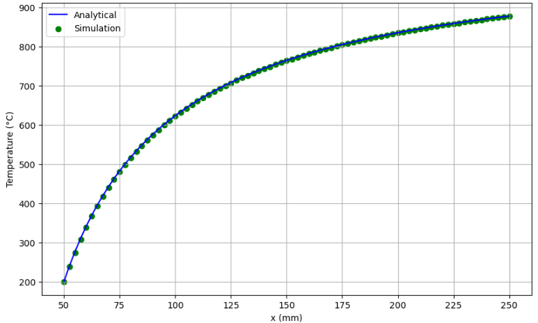
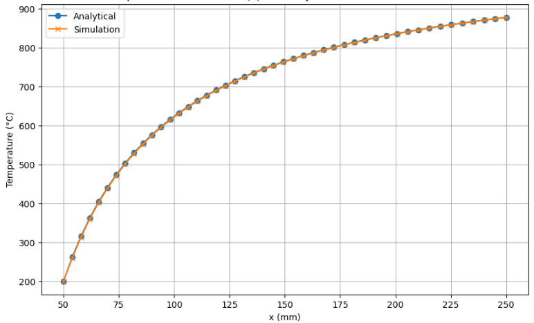
The following graph compares the analytical and simulation temperature distributions along the X-axis for the 3D conical model. The simulation results are in agreement with theoretical values.
The following graph compares the analytical and simulation temperature distributions along the X-axis for the 2D axisymmetric conical model. The simulation results are in agreement with theoretical values.