VVT23 - Radiation request using Monte Carlo, GPU view factors, and deterministic methods
| Solution | Test case | ||
|---|---|---|---|
| Finite volume method | Deterministic | SVTEST224 | |
| Monte Carlo | SVTEST225 | ||
| GPU Computed View Factors (GPUVF) | SVTEST272 | ||
| Finite element method | Deterministic | SVTEST254 | |
| Monte Carlo | SVTEST255 | ||
| GPU Computed View Factors (GPUVF) | SVTEST273 | ||
Description
The purpose of this test case is to compare computation methods when solving a radiation request model using the statistical Monte Carlo, the GPU-based View Factor (GPUVF), and the analytical deterministic view factor methods. The analytical method uses exact calculations when no shadowing is present and applies the Nusselt sphere approach when shadowing occurs. The nodal temperature and view factor results computed by the thermal solver are compared.
Geometry
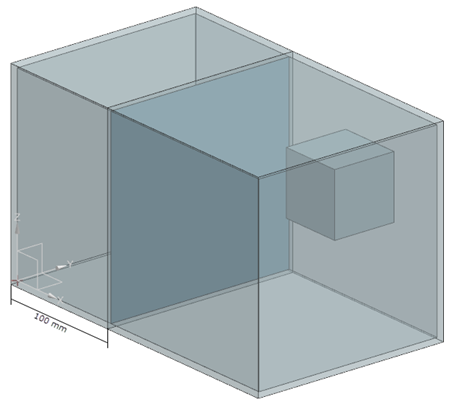
The geometry consists of a shell block with an immersed cube. The block is partitioned in two volumes with a thin shell surface. The shell block is 250 mm in length, 150 mm in width, 150 mm in height, and has a thickness of 3 mm. The thin shell surface has 1 mm in thickness and located on the distance of 100 mm from the YZ plane along the length. The immersed cube is 50 mm in length with the center located at X=205 mm, Y=105 mm, and Z=105 mm.

Simulation model
This model uses the Advanced Thermal solution type.
The block, including the inner and outer shell, and the middle surface are meshed with a 2D triangular mesh with a 20 mm element size. The immersed cube is meshed with 2D triangular elements of 15 mm size using the subdivision method.
The following material properties are used:
- Mass density: ρ = 1 kg/m3
- Thermal conductivity: k = 10 W/m·K
The emissivity of the inner shell block, shell cube block and the middle surface faced to the cube is equal to 1. The surfaces radiate from the top. The emissivity of the middle surface that is not faced the cube is equal to 0.5 and radiates from the bottom.
The following boundary conditions are applied:
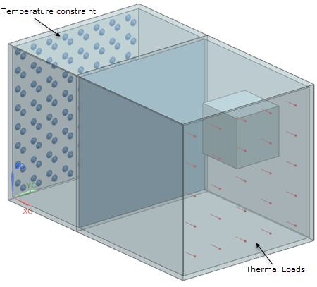
- Thermal Loads on the internal face of the block with a heat load of 10 W.
- Temperature constraint on the opposite internal face of the block with a temperature of 25 °C.
- Radiation on the 17 internal walls, including internal
block faces, middle surface and external faces of the cube using different
calculation methods:
- Deterministic with element subdivision equals to 3.
- Monte Carlo with defined Monte Carlo Setting modeling object with the Calculate View Factors only check box selected.
- GPU Computed View Factors with 15 000 number of rays. This model is computed using a graphics processing unit (GPU) with an NVIDIA Quadro P2000 graphics card enabled, and the View Factors GPU check box selected in the Parallel Configuration File in the Solution dialog box.

Theory
The Monte Carlo method computes radiative exchange by launching rays from defined solar and IR spectrum sources and tracing the rays to extinction, taking into account absorption, diffuse and specular reflection, and transmission. With the selected view factor calculation option, the thermal solver initially computes the black body view factors assuming the body is perfectly black. Then, it adjusts them to account for the actual surface properties, resulting in gray body view factors.
The GPUVF method also uses the Monte Carlo method, but is optimized to compute the radiative view factors on the GPU, which is much faster for ray tracing calculations.
Results
The following table compares the average temperatures of the six inner faces of the block using the Monte Carlo, GPUVF, and analytical deterministic methods.
| Finite volume method | Finite element method | |||||||||
|---|---|---|---|---|---|---|---|---|---|---|
| Face | Tavr (°C), Monte Carlo | Tavr (°C), GPUVF | Tavr (°C), Det | Error (%) MC/Det | Error (%) GPUVF/Det | Tavr (°C), Monte Carlo | Tavr (°C), GPUVF | Tavr (°C), Det | Error (%) MC/Det | Error (%) GPUVF/Det |
| YZ at X=0 mm | 25 | 25 | 25 | 0 | 0 | 25 | 25 | 25 | 0 | 0 |
| YZ at X=250 mm | 105.222 | 107.851 | 107.857 | 2.44 | 0.01 | 105.112 | 106.625 | 106.62 | 1.416 | 0 |
| ZX at Y=0 mm | 67.3885 | 68.461 | 68.4732 | 1.58 | 0.02 | 65.995 | 65.975 | 66.995 | 1.492 | 0.03 |
| ZX at Y=150 mm | 67.4042 | 68.467 | 68.4706 | 1.56 | 0.01 | 66.022 | 65.997 | 66.993 | 1.450 | 0.01 |
| YX at Z=0 mm | 67.3971 | 68.459 | 68.4731 | 1.57 | 0.02 | 66.019 | 65.994 | 66.994 | 1.455 | 0 |
| YX at Z=150 mm | 68.3982 | 68.470 | 68.4706 | 0.11 | 0 | 66.015 | 65.997 | 66.994 | 1.462 | 0 |
The following table compares the minimum, maximum, and average view factors sum for the Monte Carlo, GPUVF, and deterministic methods. The results are similar with finite volume and finite element methods.
| View factor sum | Monte Carlo | Deterministic | GPUVF | Error (%) MC/Det | Error (%) GPUVF/Det |
|---|---|---|---|---|---|
| Minimum | 0.993665 | 0.998014 | 0.9864 | 0.50 | 1.16 |
| Maximum | 1.10793 | 1.00086 | 1.0139 | 10.7 | 1.3 |
| Average | 1.05713 | 0.999951 | 0.9998 | 5.8 | 0.02 |
