VVT3 - Radiation between two perpendicular surfaces
| Solution | Test case | ||
|---|---|---|---|
| Finite volume method | Deterministic | SVTEST3 | |
| GPU Computed View Factors (GPUVF) | SVTEST278 | ||
| GPU Computed Ray Tracing (GPURT) | SVTEST279 | ||
| Finite element method | Deterministic | SVTEST229 | |
Description
The purpose of this test case is to determine the temperature of an insulated surface that exchanges radiant heat with an isothermal surface and the surrounding environment.
Geometry
The model is sufficiently simple, no part geometry is necessary.
Simulation model
The mesh of elements (1) and (2) is made of quadrilateral null shell element with dimensions of 0.5 m by 0.5 m. The top surface emissivity of the element (1) is 0.6 and element (2) is 1.
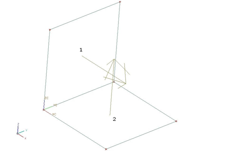
The two-element mesh has no material and physical properties assigned to it. Consequently, the thermal conductivity is zero, which is of importance for this activity in order for radiant heat exchange to be the main heat transfer mechanism.
The following boundary conditions are applied:
- Temperature constraint on the element (1) with a value of T1 =1000 K.
- Radiation: Radiation Enclosure on
the top-side region with selected Include Radiative
Environment using different calculation methods:
- Deterministic with element subdivision equal to 5.
- GPU Computed View Factors with 15 000 number of rays.
- GPU Computed Ray Tracing with 15 000 number of rays.
The following solution options are set:
- Solution Type=Steady State
- Results Options: Select view factor sums, net radiative fluxes, radiosity fluxes and irradiance fluxes. The radiative environment temperature is set to T3 = 300 K.
- This model is computed using a graphics processing unit (GPU) with an NVIDIA Quadro P2000 graphics card enabled, and the View Factors GPU check box selected in the Parallel Configuration File in the Solution dialog box.
The default solver parameters are selected.
Theory
The following thermal circuit diagram [19] shows the radiation heat transfer of three surfaces: surface (1), insulated surface (2) and room at 300 K (3).
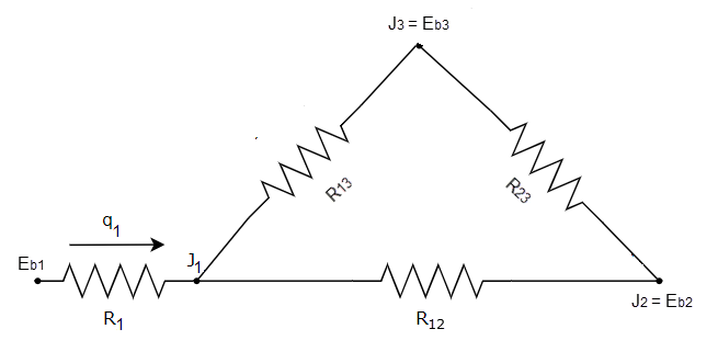
Because the surface (2) is an insulator, it has zero heat transfer, therefore J2 = Eb2.
J3 = Eb3 because the room is large and R3 approached zero.
The view factor between surfaces (1) and (2) is F12 = F21 = 0.2. Since surfaces elements (1) and (2) are convex, F11 = F22=0 and by the enclosure identity, F13 = 1 - F12 = F23 = 0.8. Radiant heat exchange for this system can be modeled using a resistive network. The surface resistance of surface (1) is defined as:
The remaining resistances are given by:
The equivalent resistance of the network is:
The blackbody emissive power of surface (1) is given by the Stefan-Boltzmann law:
while that of the surroundings is Eb3 = 459.2 W/m2. Then, the overall heat transfer rate through the network is defined as:
The radiosity for the surface (1) is
while the radiosity of surface (2) is obtained realizing that there is zero net heat flow at that surface:
Finally, because surface (2) is an insulator, J2 = Eb2 and by the Stefan-Boltzmann law again, T2 = 599.38 K.
The irradiance for the surface (1):
The net radiative flux for the surface (1):
Since the surface (2) is the blackbody and net radiative flux is equal to 0, the irradiance is then equal to qin = 7316 W/m2.
Results
The following table compares the thermal solver results calculated using both finite volume and finite element discretization methods with the theoretical results. A good agreement is found.
| Finite volume method | Finite element method | ||||||||
|---|---|---|---|---|---|---|---|---|---|
| Parameter | Theory | Det | Error (%) Det | GPUVF | Error (%) GPUVF | GPURT | Error (%) GPURT | Det | Error (%) |
| T2 (K) | 599.38 | 599.82 | 0.07 | 599.07 | 0.05 | 599.81 | 0.07 | 599.8 | 0 |
| J1 (kW/m2) | 34.746 | 34.74 | 0.018 | 34.740 | 0.018 | 34.780 | 0.097 | 34.775 | 0.09 |
| J2 (kW/m2) | 7.316 | 7.302 | 0.199 | 7.302 | 0.199 | 7.338 | 0.29 | 7.338 | 0.30 |
| q1,in (kW/m2) | 1.830 | 1.903 | 3.95 | 1.821 | 0.486 | 1.828 | 0.096 | 1.903 | 3.95 |
| q2,in (kW/m2) | 7.316 | 7.338 | 0.292 | 7.301 | 0.20 | 7.337 | 0.287 | 7.338 | 0.976 |
| q1,net (kW/m2) | 32.915 | 32.920 | 0.013 | 32.920 | 0.013 | 32.920 | 0.013 | 32.870 | 0.139 |