Configure thermal solver settings
Learn how to configure thermal solver settings, modify time stepping options, evaluate accuracy versus solve time, run coupled thermal-structural solutions, post-process cyclic symmetry results, and control output settings.
Introduction
In this tutorial, you will:
- Modify time stepping options.
- Evaluate the impact on solution accuracy and solve time.
- Understand solver communication frequency and results output settings.
- Post-process cyclic symmetric geometries.
- Run a combined transient and steady-state analysis.
Load the thermal plugin
Enable the ExpressionsPlugin.dll if not already active. The predefined boundary conditions in the model use heat transfer coefficient (HTC) correlations implemented through custom expressions. These correlations require the plugin to evaluate correctly during the simulation.
- Choose .
- Click Simulation, expand Pre/Post, and scroll to Expressions.
- On the Plugin tab, select the Use Custom Plugin check box and in Custom Plugin, type the full path to the ExpressionsPlugin.dll file, as plugin\ExpressionsPlugin.dll.
- Click OK, exit Simcenter 3D, and restart the application to activate the plugin.
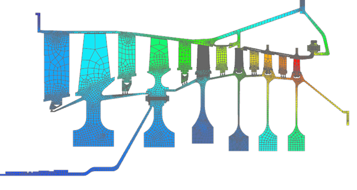
Define assembly load options
Configure search folders to load a model whose part and FEM files are stored in multiple directories.
-
On the Home tab, click Assembly Load
Options
 .
.
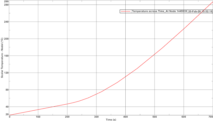
Inspect solver and time step settings
Review thermal solution controls and time step definitions.
-
In the Post Processing Navigator, expand and double-click Temperature -
Nodal.
-
Choose
 .
.
-
Select Across Iterations, set
Method to By Node ID, and
in the Nodal Label box, type
1449939.
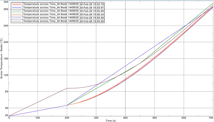
This generates a temperature graph at the selected node, which will be used in the next steps to compare results from solutions with modified time stepping.
Modify time step options and compare results
Evaluate solution accuracy and solve time sensitivity to time stepping controls. Time step size affects both convergence and accuracy. If too few time steps are used, the solution may not converge or may miss important transient behavior, such as temperature spikes. A proper balance between time step size and convergence tolerance is required to obtain accurate and stable results.
-
In the Post Processing Navigator, for each solution
under the Graph node, right-click
Temperature across Time and select
Overlay to overlay three graphs on the same
window to compare accuracy.
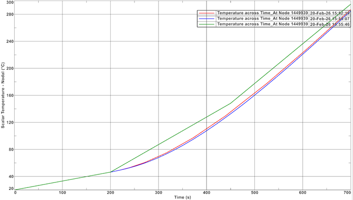
Observe that the temperatures at 700[s] for the Automatic time stepping models differ by approximately 2 °C, while the very coarse time step approach results in an error of about 10 °C.
Run a coupled thermal-structural solution
Activate structural coupling and review coupled solution parameters.
-
On the Solution Control tab, in the
Coupled Control group, next to Coupled
Solution Parameters click
 .
.
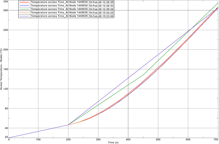
Modify results output options
Control solver output times and reduce result file size.
-
Solve and overlay the nodal temperature at node
1449939 for all thermal solutions to compare
results.
Notice the Reduced_Output curve is straight, and the endpoint aligns with the Thermal_Refine_Mod solution.
Create a combined steady-state and transient run
In some cases, it is useful to combine steady-state and transient analyses. For example, you may want to begin from a steady-state full-power condition and then simulate a transient shutdown. Modify one step of the transient solution to run as steady state and observe how this change affects the results.
-
Solve and compare results to previous transient-only solutions.
Additional notes
- Review additional advanced parameters in the advanced parameters catalogue.
- Refer to the thermal solver reference manual for detailed documentation.