Solution monitor
This topic explains how to monitor thermal and structural solutions, interpret solver modules and convergence graphs, and track warnings, errors, and solution progress during the analysis.
This lesson may include hands-on exercises. Review the Discussion section for background information or click the button to proceed to the practical section.
Discussion
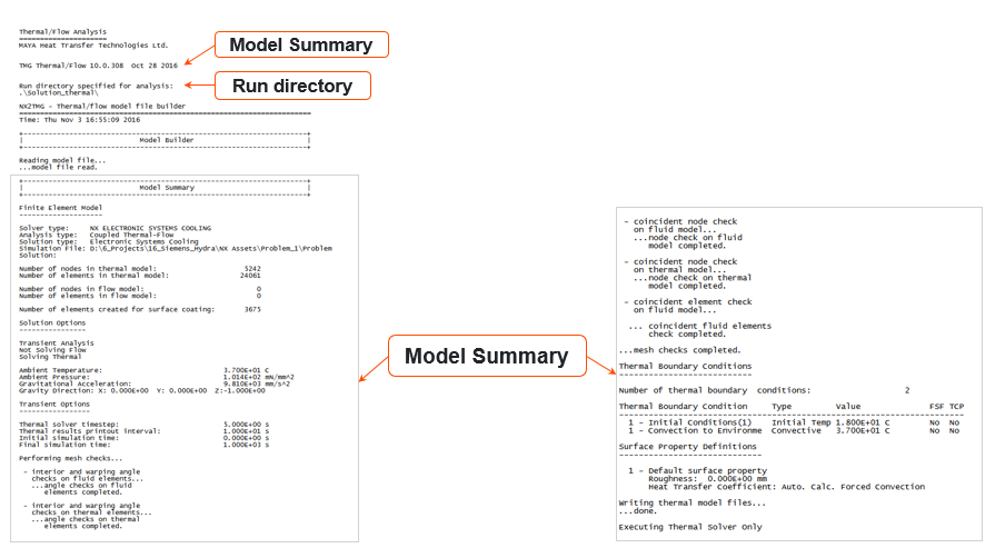
The Solver Monitor provides information from the solver during the analysis. You can track:
- Solver version, run time, and run directory.
- Model summary.
- Solution status and the current thermal solver module being executed.
- Convergence residuals at each iteration during the analysis.
- Warnings and error messages.
You can abort or stop a solution. The Solver Monitor parses relevant data from the .f06 file for the structural solution.
- Thermal solver modules in the log file
- The Solver Monitor information is saved to:
<simulation/model name>-<solution/analysis
name>.log
The following table describes the thermal solver modules:
Input Executable Module description Output INPF MAIN Module Performs data checking, determines which modules to run. <simulation/model name>-<solution/analysis name>_verbose.log INPF DATACH Module Performs data checking and orbit creation. <simulation/model name>-<solution/analysis name>_verbose.log <simulation/model name>-<solution/analysis name>_report.log
tmggeom.dat
INPF tmggeom.dat
ECHOS Module Calculates each element CG, element center, area or volume, hydraulic diameter, and surface normal along with the location of the nodes. VUFF tmggeom.dat
INPF tmggeom.dat
COND Module Calculates capacitances, hydraulic resistances, and conductive conductances from geometry. MODLF tmggeom.dat
INPF tmggeom.dat
VUFAC Module Calculates view factors, heat flux view factors, thermal couplings from geometry (optional). MODLF VUFF
<simulation/model name>-<solution/analysis name>_verbose.log
<simulation/model name>-<solution/analysis name>_report.log
INPF tmggeom.dat
VUFF
GRAYB Module Calculates radiative conductances and gray body view factor matrices from view factors. VUFF MODLF
tmggeom.dat
VUFF INPF
tmggeom.dat
POWER Module Calculates IR and solar spectrum heat loads from view factors and gray body view factor matrices. VUFF MODLF
INPF MODLF
tmggeom.dat
MEREL Module Performs model simplification, merging, substructuring, and combines parameters calculated from geometry and defined on Card 9. <simulation/model name>-<solution/analysis name>_report.log MODLCF
tmggeom.dat
USER1 MODLCF
tmggeom.dat
ANALYZER Module Calculates temperatures and total pressures. <simulation/model name>-<solution/analysis name>_report.log TEMPF
PRESSF
tmggeom.dat
tmgrslt.dat tmggeom.dat
RSLTPOST Module Transforms results into binary files. Multiple <name>.unv files or one <name>.bun Data available from ANALYZER POSTLIB Writes results into binary universal format. POSTLIB is a post-processing library used by ANALYZER and has direct access to the analysis result data.
<name>.bun - Solution Monitor graphs
- Multiple graphs are available to track the solution progress. The
Time Step Convergence graph is used to:
- View how far the convergence ratios are from the criteria. Tighten or loosen the convergence criteria to improve convergence behavior.
- View convergence trends. Sometimes, the errors have a downward trend, but the solution does not have enough iterations to reach the specified criteria.
The Cumulative Iteration History graph is used to:
- Evaluate whether the time-step size is adequate. Too many bisections of the time step are inefficient, and may indicate that a smaller time step would be more effective.
- Identify when convergence becomes more challenging because of abrupt boundary-condition changes, such as a change in contact status. In this case, it may be useful to create a new solution step with finer time increments.
Hands-on material
To gain experience with the topics discussed here, complete the following: