Set up a CubeSat thermal analysis from start to finish
This is an objective-based exercise. Instead of being provided a list of instructions, you are simply provided a scenario and problem statement to solve.
If you encounter difficulties while following the steps, refer to the Answer video: Set up a CubeSat thermal analysis from start to finish.
![]() Download and extract the part
files.
Download and extract the part
files.
Scenario:
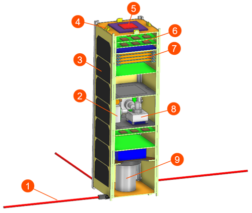
You are a thermal engineer working on a 3U Earth observation CubeSat mission in low Earth orbit at an altitude of 400 km.
- Antennas (1) for communication with the ground.
- Reaction wheels (2) that provide precise attitude control.
- Solar panels (3) mounted on four sides, each containing seven panels that generate electrical power.
- Sun sensors (4) that measure the Sun’s direction to determine the spacecraft’s attitude.
- GPS antenna (5) to determine the satellite position in orbit.
- Printed circuit boards (PCBs) (6) that host the spacecraft’s electronics and dissipate heat.
- Batteries (7) that store electrical power for spacecraft operation.
- Magnetorquer (8) that control attitude using Earth's magnetic field.
- Observation camera (9) that captures images of the Earth.
The spacecraft operates in low Earth orbit, where it is exposed to solar radiation, reflected radiation from Earth (albedo), Earth infrared radiation, and deep space cooling. At the same time, internal components generate heat that must be properly dissipated.
The mission team must ensure that all critical components operate within their allowable temperature limits throughout the orbit:
- Battery: 5 °C to 25 °C
- Payload (camera): −10 °C to 25 °C
- Solar cells: −50 °C to 100 °C
Objectives:
You must determine whether the CubeSat design maintains all critical components within their allowable temperature ranges under realistic orbital conditions.
To complete the analysis, you will:
- Create and use a custom FEM template with predefined material and thermo-optical properties.
- Generate FEM models for all major components.
- Mesh components using different techniques such as 3D, 2D, or simplified representations, depending on geometry complexity and required thermal accuracy.
- Assign appropriate material and thermo-optical properties to each component.
- Simplify selected components using idealized geometry by removing features that do not significantly affect the thermal results but increase the element count.
- Assemble the full model and define thermal contacts between components.
- Apply orbital heating conditions.
- Define space radiation to a deep space environment at 4 K.
- Apply internal heat loads from electronics and batteries.
- Run a transient solution.
- Post-process results to evaluate temperature distribution and heat flux.
- Compare the predicted temperatures against allowable limits to determine whether the design meets thermal requirements.
Instructions:
Create a custom template
Template files store the analysis settings and FE modeling definitions used to create a new FEM or Simulation file. The .pax file is an XML file that lists the FEM and Simulation templates that the software loads automatically when you create a new part file from a template.
-
Update the
<Filename>value to point toSST_CustomTemplate.femand the<Presentation>name toSST‑Custom Template.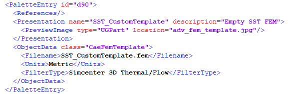
Alternatively, you can redirect the default template directory to your current working folder to avoid modifying the default templates. To do this, set the UGII_TEMPLATE_DIR variable environment to the working folder. For more information, see the Automate meshing with selection recipes and template files tutorial.
Generate FEM models
Mesh the parts
- Use 3D meshes for thermally critical or volumetric components, for example, battery and structure.
- Use 2D shell meshes for thin structures.
- Use idealized geometry or primitives for simplified representations.
-
For each FEM file listed in the table, create a 3D Swept
Mesh with a 10 mm element size. Apply the material and
thermo-optical properties specified in the following table.
When you create Solar_Panel_fem1.fem, set Polygon Body Resolution to High.
FEM Material properties Advanced Thermo-Optical properties Side_fem1.fem Create a new aluminum material with mass density of 2700 kg/m3, a thermal conductivity of 157 W/(m·K), and a specific heat of 929 J/(kg·K). Create a new thermo-optical property with emissivity and absorptivity set to 0.88. Solar_Panel_fem1.fem Note:Set % of Element Size to 0.PCB (generic) Solar Cells Bottom_Plate_fem1.fem Aluminum Bare Aluminum PCB_fem1.fem Note:Mesh the board only; do not mesh components.
PCB (generic) PCB End_Plate_fem1.fem Aluminum White Paint - States -
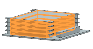
Use a more detailed 3D mesh for the battery since it is a thermally
critical component because its temperature must stay within a narrow range
and directly impacts mission safety. Create a 3D Swept
Mesh with a 10 mm element size as shown in the table:
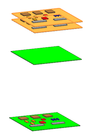
Category PCBs Cells Connector Spacers Selection 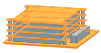
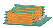
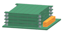
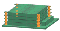
Properties Material: PCB (generic) Thermo-optical properties: PCB
Material: Invar Thermo-optical properties: PCB
Material: PCB (generic) Thermo-optical properties: Black Paint
Material: Stainless Steel Thermo-optical properties: Bare SS
-
For camera, use mixed meshing 3D and 2D shell to balance accuracy and
performance as shown in the table:
Category Board Spacers Camera Box Selection 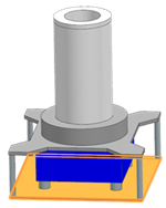
Properties 3D Swept Mesh with a 10 mm element size. Material: PCB (generic)
Thermo-optical properties: PCB
3D Swept Mesh with a 10 mm element size. Material: Stainless Steel
Thermo-optical properties: Bare SS
3D Hex Dominant Mesh with a 10 mm element size. Material: Aluminum
Thermo-optical properties: Iridite
2D Mesh QUAD 4 Thin Shell with 10 mm. Set Thickness is 2 mm
Material: Aluminum
Thermo-optical porperties: Top is set to Black Paint, Bottom is set to Bare Aluminum
-
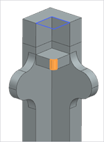
For parts where only mass representation is required and geometric detail
is not needed, use primitives instead of meshing the full geometry. In
Wheel.prt, create a primitive using the
Extrude command. To do this:
- Select the indicated face and extrude a box sized to preserve
approximately the same radiating surface area.
- Create a new FEM file, set Bodies to Use to Select and choose only the box.
Alternatively, you can create a new FEM file for Wheel.prt and represent it as a box using .
- Select the indicated face and extrude a box sized to preserve
approximately the same radiating surface area.
-
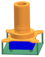
Remove unnecessary details, such as small chamfers and faces on both sides
of the rail using Delete as shown:

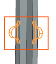
7 faces selected
2 faces selected
32 faces selected
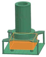
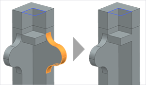
-
Use the Replace command to remove the faces on the
ends of the rail, as shown.
Simulation setup
-
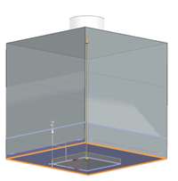
Define orbital heating to apply solar flux, albedo, and Earth IR using the
Orbital Heating simulation object with the
following settings:
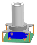
- The Illuminate Selected Elements type.
- For Top Side Illuminated Region, select the
following 54 external faces that receive the sun light. You can
ignore small faces for this tutorial.
- GPU Computed Ray Tracing calculation method.
- Number of rays is 15000.
-
Define the classical Orbit using the following
settings:
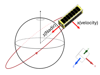
- For the spacecraft orientation, set the first vector point toward
Nadir, since the camera faces the Earth,
and align the second vector with the X velocity vector, as
shown.
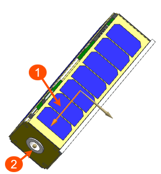
- The CubeSat rotates about its own axis. Specify the indicated vector
(1) and point (2), and set the rotation to 360° over one
orbit.
- For the Sun planet characteristics, compute the solar flux for the December solstice Sun position and specify the solar flux in W/m2.
- For the orbit parameters, specify:
Minimum altitude: 400 km Orbit inclination: 25° 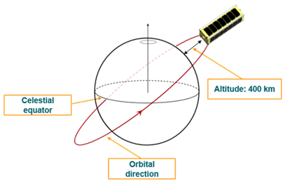
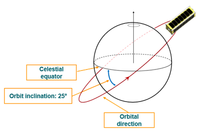
- Set 12 intervals to calculate the satellite positions along the orbit. Increasing the number of intervals increases the solution time.
- For the spacecraft orientation, set the first vector point toward
Nadir, since the camera faces the Earth,
and align the second vector with the X velocity vector, as
shown.
-
Apply heat loads using Thermal Loads on the
following components:
- 1 W on the first PCB board and 2W on the second PCB board.
- 3 W on the battery cells.
- 1 W on the first PCB board and 2W on the second PCB board.
-
Edit and set up a transient solution using the following parameters:
- Set the solution end time based on the orbit period.
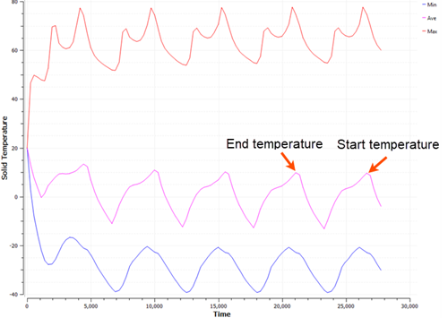
- Enable periodic convergence and instruct the solver to stop the
solution when the temperature change between orbits is less than 1
°C.
The solver compares the temperatures at the start and end of the orbit. If the difference is within the specified tolerance, it stops the solution.
- Use a constant time step of 60 s.
- Request 20 results per orbit and save results for the last orbit only.
Review results
-
Display the temperatures for battery, and compare the temperatures against
allowable limits to determine whether the design meets thermal
requirements.
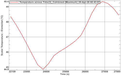
The temperature range is 28–49 °C, which falls outside the allowable range of 5–25 °C. The design does not meet thermal requirements and requires modification, such as adding heaters or changing material properties.
-
Display the battery temperatures for the last orbit and plot the graph
across iterations.