Set up a CubeSat analysis with heater sizing using primitive geometries

This is an objective-based exercise. Instead of being provided a list of instructions, you are simply provided a scenario and problem statement to solve.

You will learn how to set up a CubeSat thermal analysis using primitive shapes. You will build a simplified thermal model, define conductive and radiative heat transfer, simulate orbital conditions, and size a heater to maintain the battery within its allowable temperature range.

If you encounter difficulties while following the steps, refer to the Answer video: Set up a CubeSat analysis with heater sizing using primitive geometries.

Scenario:

You will develop a preliminary thermal model of a CubeSat during an early design study. To reduce modeling effort, you will represent the spacecraft using primitive geometries instead of detailed CAD.

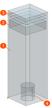
The CubeSat includes:

A structural body (1) representing the satellite walls.
An internal battery (2), which is thermally critical.
Two PCB boards (3) that dissipate heat.
A camera (4) that points toward Earth.

The CubeSat operates in low Earth orbit and is exposed to solar radiation, Earth infrared radiation, and deep space cooling. During eclipse, the CubeSat loses heat to space through radiation, which can cause the battery temperature to drop below its allowable limit.

Objectives:

Your main objective is to maintain the battery temperature between 19 °C and 22 °C during operation. To achieve this, you will simulate a worst-case cold scenario by selecting orbital conditions that maximize eclipse duration. You will then estimate the heater power required and implement thermostat-controlled heating.

To complete the analysis, you will:

Build a simplified CubeSat geometry using primitive shapes.
Mesh the model and assign material and thermo-optical properties.
Represent the battery thermal mass using a lumped (0D) element.
Define radiation and orbital heating boundary conditions.
Create conductive thermal couplings between components.
Run a worst-case cold orbital scenario (beta angle = 0°).
Estimate the required heater power using a temperature constraint.
Size the heater based on the estimated power.
Replace the temperature constraint with a heater and thermostat control.
Evaluate the thermostat behavior and battery temperature response.

Instructions:

Create a new part file and name it as cubesat.prt.
In the Modeling application, create a block with a length of 100 mm, width of 100 mm, and height of 330 mm to represent the CubeSat body.
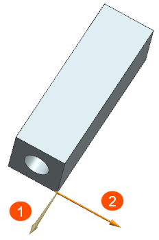
On the bottom face of the block, create a cylinder to represent the camera with the following parameters:
- Set the vector as shown:
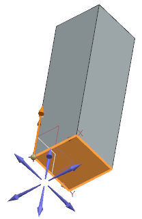
- To define the point, use the Between Two Points option and select the opposite points of the block.
- Set the diameter and height to 50 mm.
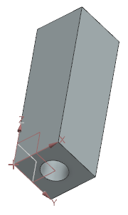
- Subtract the cylinder from the block. The cylindrical surface represents the camera lens.
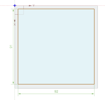
To represent a battery in the middle of the CubeSat body, create the geometry using the Extrude command. Create a rectangular on the block surface as shown.
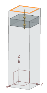
Extrude it using the following values:
- Start distance: 35 mm
- End distance: 65mm
- Reverse the direction if needed so that the created block lies inside the CubeSat body.
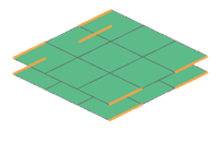
Reuse the sketch to create two PCB boards using Extrude.
To make the sketch external, in the Part Navigator, right-click Extrude and select Make Sketch External.
- For the first PCB board, set the start and end distance to 13 mm.
- For the second PCB board, set the start and end distance to 25 mm.
Save all files and close Simcenter 3D.
Add a custom template to the .pax file that includes predefined material and thermo-optical properties by editing the XML content with a text editor and adding entries that reference your custom FEM template file.
The .pax file is an XML file that defines the FEM , Simulation, and assembly FEM file templates that the software loads automatically.
Download the cubesat_primitives\Template folder, which contains the .pax file and FEM template files.
The Automate meshing with selection recipes and template files tutorial explains how to add a custom template.
Open the created part file.
In the Pre/Post application, create a new FEM file in the Simcenter 3D Space Systems Thermal environment, using the SST -Custom Template.
Mesh the camera lens, camera walls, CubeSat walls, battery walls, and PCBs using the 2D Mesh with QUAD 4 Thin Shell type and a 30 mm element size.

For each mesh, create a separate mesh collector and set the following properties:


Category	Camera lens	Camera walls	CubeSat walls	Battery walls	PCB boards
Material	PCB (generic)	Stainless Steel	Aluminum	Null Shell	PCB (generic)
Thickness	5 mm	5 mm	5 mm	N/A	2 mm
Thermo-optical properties	Solar Cells to the top and bottom radiation	Iridite to the top and bottom radiation	Create new thermo-optical properties with emissivity and absorptivity of 0.88. Set to the top and bottom radiation.	Silver Teflon - States to the top and bottom radiation.	PCB to the top and bottom radiation

To account for the battery mass, use the OD lump element mass in the middle of the box. To do this:
- Add a point in the middle of the box using the Between Two Points type.
- Mesh the point using 0D Mesh with the Lump type.
- Assign the Aluminum material to apply heat capacity.
- Set non-structural mass to 0.8 kg.
- There is no radiation.
Name the point as a Battery_mass by right-clicking it and selecting Properties.
In post processing , it will give us a 0D mass temperature of the point automatically. The solver interpolates the temperature from the closest elements.
Use Model Display Preferences to display the mesh based on mesh collectors.
Create a Simulation file using the Simcenter 3D Space System Thermal environment.
Create a transient solution and define the following settings:
- Set the run directory to Solution Name.
- If you want to use GPU-based radiation, configure it in the Parallel Configuration Tool by selecting the GPU to use for radiation calculations.
- Set the solution units to meters.
- Set the space environment temperature to 4 K.
- Select the Thermal Connections results option to review how the thermal couplings are connected.
Create groups for the lens, lens walls, CubeSat walls, battery, and PCBs on the geometry for post processing. You will use these groups later to review the temperature for each group in the data.html file.
Defining the groups on the geometry ensures the selections persist after remeshing.
Create radiation boundary conditions between each surfaces and space using the All Radiation type. Select any calculation method. For this example, the Deterministic method is used because the model is simple.
Define orbital heating to apply solar flux, albedo, and Earth IR using the Orbital Heating simulation object with the following settings:
- The Illuminate Selected Elements type.
- For Top Side Illuminated Region, select the external faces that receive the sun light.
- Select any calculation method. For this example, the Deterministic method is used.
  Note:
  If you use a GPU-based method for radiation, you must also use a GPU-based method for orbital heating.
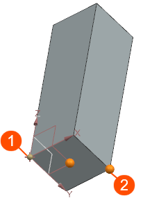
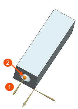
Define the beta angle Orbit using the following settings:
- For the spacecraft orientation, set the first vector (1) point toward Nadir, since the camera faces the Earth, and align the second vector (2) with the -X velocity vector, as shown.
- The CubeSat rotates about its own axis. Specify the indicated vector (1) and point (2), and set the rotation to 360° over one orbit.
- For the Sun planet characteristics, compute the solar flux for the June solstice Sun position, where the lowest sun flux and specify the solar flux in W/m².
- Set the beta angle to 0° to maximize the eclipse duration and run the worst-case cold scenario for heater sizing.
- Altitude is 400 km.
Visualize the orbit using the Orbit Visualizer command.
Confirm that the Sun beta angle is 0° and ensure that the satellite rotates as defined.
Create thermal contacts between the satellite walls, battery and PCBs, using Thermal Coupling.
- For the battery and satellite walls coupling, select four battery walls that are connected to the CubeSat sides as a primary region, and four satellite walls as a secondary region, and set total conductance to 10 W/°C. Select the Projective Intersection method and select the Show Ancillary Display to inspect the thermal connections before solving.
- For the battery walls and the 0D lamp element, select 6 battery faces as a primary region, and the mass point as a secondary region and set total conductance to 1000 W/°C. Clear the Only Connect Overlapping Elements check box to connect every primary battery element to the 0D element.
- For the PCBs and satellite walls, select eight element edges at the PCBs corners as a primary region, assuming the mounting points at these corners.
  
  Select two corresponding satellite walls as a secondary region, and set total conductance to 0.1*8 W/°C bolted connections. Clear the Only Connect Overlapping Elements check box.
To size a heater, define a temperature sink by applying a Temperature constraint of 20 °C to the battery 0D element to estimate the required heater power.
The solver enforces this temperature and reports the heat flow required to maintain it.
Add the DISPLAY BC SUMMARY TABLE and PLOT BC SUMMARY advanced parameters to generate the <simulation_name>-<solution_name>.bcda and <simulation_name>-<solution_name>_data.html files, where you can inspect various result quantities associated to boundary conditions, thermal couplings, and named points.

Note:
Starting with release 2606, the solver creates these files in the run directory by default without requiring the advanced parameters.
Edit and set up a transient solution using the following parameters:
- Set the solution end time based on the orbit period.
- Enable periodic convergence and instruct the solver to stop the solution when the temperature change between orbits is less than 0.1 °C. The solver compares the temperatures at the start and end of the orbit. If the difference is within the specified tolerance, it stops the solution.
- Use a constant time step of 60 s. Do not use a time step greater than 60 s, as this increases the solution run time.
- Request 50 results per orbit and save results for the last orbit only.
Solve the solution.
Inspect the log file.
In the Heat Flow Load summary, next to the temperature constraint, notice how much heat is dissipated at specified time.
In the Post Processing Navigator, click Thermal Connections to display the lines representing heat paths created by the thermal solver between primary and secondary elements of supported thermal couplings. Verify that the elements are connected correctly.
Open the simulation name-solution name_data.html file in the run directory and review the heat flow from the battery to the satellite walls.
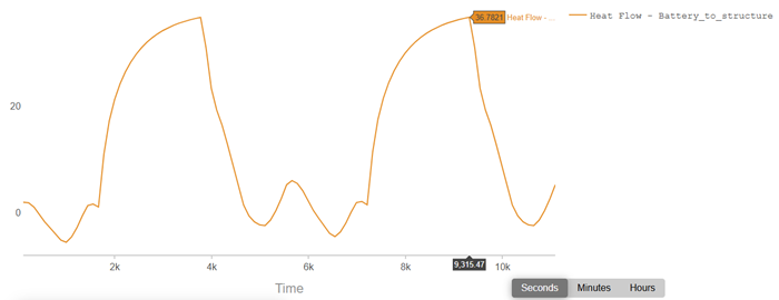
Use this information to estimate the power required to maintain the battery at 20 °C. The required power ranges from 6 to 36 W. To have less duty cycle, you will set the heater size to 40 W.
Clone the solution.
Remove the temperature constraint.
Add a heater to the battery by applying a Thermal Load of 40 W to the battery mass, and define a Thermostat with a sensor on the battery mass to control the temperature between 19 °C and 22 °C.
Solve the cloned solution.
Open the new simulation name-solution name_data.html file and display:
- Battery temperatures, which varies between 19 and 22 °C.
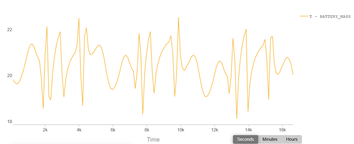
- Heat flow for the battery to the satellite walls.
  
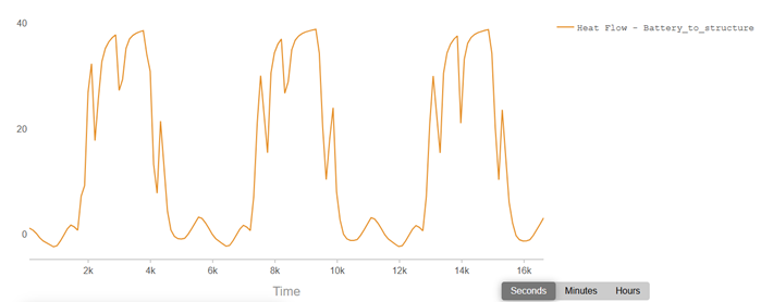
  Notice how the thermostat cycles on and off during the simulation.
- Minimum and maximum temperatures for the different components.
Open the simulation name-solution name_ThermostatsReport.csv file to view the sensor temperature, when the thermostat turns on and off, and the amount of heat applied.
Open the Thermostat_report.log file to review the thermostat duty cycle. You can view:
- How much times the thermostat turns on.
- Duty cycle.
- Average power of heaters.