Map metal temperatures from WEM to component models

Learn how to map metal temperatures from a Whole Engine Model (WEM) to component models. This workshop covers rotational periodicity mapping, axisymmetric mapping, alignment tools, merged mapping solutions, and automatic generation of Nastran and ANSYS outputs.

Download and extract the part files.

Introduction

Metal temperatures are commonly mapped from the Whole Engine Model (WEM) to component models for structural stress analysis. Using the dedicated mapping solution in Simcenter 3D, users can control translational and rotational offsets and map temperatures between 2D and 3D models with different mesh types, sector angles, and orientations.

With the merge results functionality, temperatures can be:

  • Mapped from multiple source solutions.
  • Updated selectively for specific components.
  • Appended to an existing mapped solution.

Solving a mapping solution generates a BUN file, and depending on the selected options can automatically create structural solutions or solver input files.

In this tutorial, you will:

  • Set up rotational periodicity mapping.
  • Define axisymmetric mapping constraints.
  • Use the mapping alignment tool.
  • Create a merged mapping solution.
  • Automatically generate Nastran and ANSYS input files.
  • Automatically generate an ANSYS solution with temperature constraints applied.

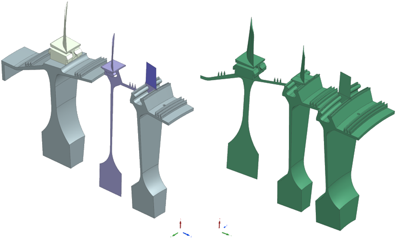
Open the source model and inspect

Inspect source solutions and understand which temperatures will be mapped.

  1. Choose FileOpen and open mapping\source\CompressorAxisymmetricsim.sim.
  2. Inspect solutions source1 and source2.
    In this tutorial, the approach is to first map the results from source1 onto the target model, and then update the temperature of disk 2 using results from the source2 solution. In this example, both source solutions share the same mesh. However, temperature mapping can also be performed between different simulation files with different meshes. Note that the source2 model includes an additional temperature constraint (23), which modifies the temperature of disk 2.Also observe that disk 3 is modeled with cyclic symmetry.
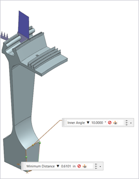
  3. Observe that there is a cyclic symmetric disk 3 in the model and measure the sector angle to confirm that it is 10 degrees.


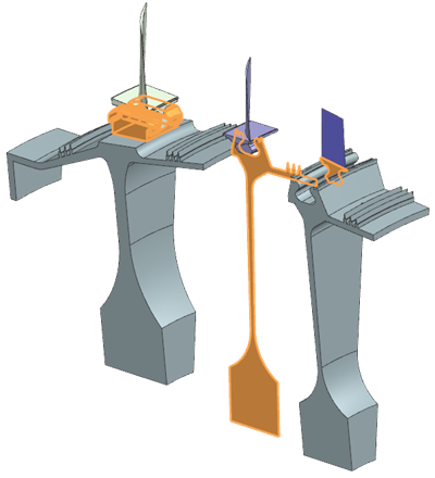
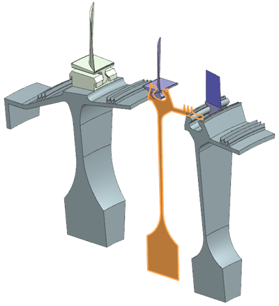
Open the target model and inspect

Review geometry differences and plan mapping strategy.

  1. Open mapping\target\target_sim1.sim.
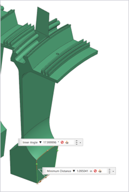
  2. Measure the cut angle of disk 3 in this model.
    Notice that the sector angle is18 degrees. Use the rotational periodicity mapping constraint to map temperatures between models with different cyclic sector sizes.

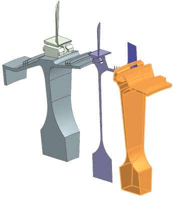
  3. Inspect the remaining components and plan the thermal mapping strategy.
    You will map disk 1 from 3D to 2D and map disk 2 from 2D to 3D. The model also includes 3D-to-3D and 2D-to-2D mapping cases. Although a single axisymmetric mapping constraint can handle all scenarios, create multiple axisymmetric mapping constraints to ensure accurate temperature transfer at component interfaces. If you use only one axisymmetric mapping constraint, the solver may not correctly determine which source components correspond to which target components at contact regions.

  4. Observe that the rotational axis differs between the source and target models: the source model uses the Z-axis, while the target model uses the Y-axis.

    Note that the axial positions of the disks differ between the source and target models. If the disks were located at the same axial position and the 2D solid options were properly defined, no manual transformation would be required.

    In this case, both an axial and a rotational offset exist. Use Source Model Mapping when setting up the target mapping solution to align the source model with the target geometry.

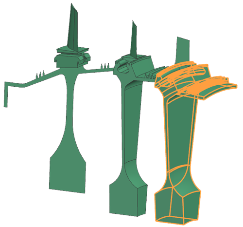
Create mapping constraints in the source model

Define rotational periodicity and axisymmetric mapping zones.

  1. Click the (Simulation) CompressorAxisymmetricsim.sim window.
  2. Activate the source1 solution.
  3. Choose Home > Loads and Conditions > Constraint Type > Mapping .
  4. From the type list, choose Rotational Periodicity Association Zone and select the shown body.


  5. In the Number of Segments box, type 36.
  6. In the Axis group, define the vector as the Z-axis, and the point as 0,0,0.
  7. Click OK.
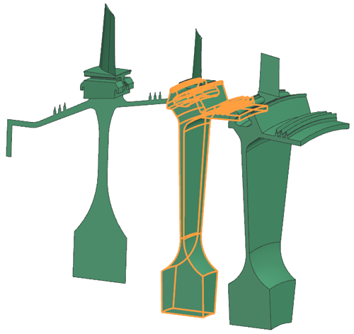
  8. Create two Axisymmetry Association Zone type mapping constraints.

    Ensure that, within each zone, the bodies are not in contact with one another. This separation is critical because the solver cannot reliably distinguish overlapping contact regions when multiple contacting bodies are included in a single source zone. If contacting bodies are grouped together, the solver may incorrectly associate source and target regions, leading to inaccurate temperature mapping. By splitting the model into multiple mapping constraints, each with non-contacting bodies, you explicitly guide the solver in establishing correct source–target relationships at the interfaces.

    First constraint (4 bodies selected) Second constraint (3 bodies selected)
    Name = Axisymmetric_1 Name = Axisymmetric_2


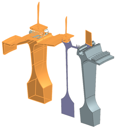
    There are 3 mapping constraints in the source1 solution.

  9. Make the source2 solution active.
  10. Create an axisymmetric mapping constraint for disk 2 and name it as Mapping_disk2.


    This will be used to update the target mapping solution disk 2 temperatures.
  11. Choose Menu > Analysis > Solve All Solutions and click OK.
  12. In the Post Processing Navigator, under the source1 solution, double-click Thermal and display the nodal temperatures at the last time point.
  13. Choose Results > View Layout > Side by Side.
  14. Display the source2 solution nodal temperature at the last time point and select the second viewport.
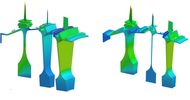
  15. Edit the legend extremes for the source2 solution so they match those of the source1 solution allowing you to compare the results directly.


    Notice the change in disk 2 temperature between the results.

Create a mapping solution in the target model

Reference source bun file and define mapping alignment.

  1. Click (Simulation) target_sim1.sim.
  2. In the Simulation Navigator, right-click target_sim1.sim and select New Solution.
  3. Make sure that Solver is set to Simcenter 3D Thermal/Flow and Analysis Type is set to Mapping.
    You can also create a mapping solution in the Multiphysics environment. However, it is suggested to use the mapping solution in the Thermal-Flow environment, as it includes the most up-to-date mapping features.
  4. Click Create Solution.
  5. On the Mapping Details page, in the Source Model Results File box, reference the BUN file of source1 from the source simulation.
    The mapping solution uses all time steps in the source BUN file by default. If you require only specific time steps, select them on the Mapping Details page in the Select Output Times field. By default, the solver limits temperature extrapolation to the element range of the source model.
  6. On the Optional Output page, clear all check boxes related to the generation of mapping outputs.
  7. Click OK.
  8. Choose Home > Loads and Conditions > Constraint Type > Rotational Periodicity Target Zone to create a mapping constraint for disk 3.


  9. Create two Axisymmetry Target Zone which correspond to the selected components in the source model.
    First target (4 bodies selected) Second target (3 bodies selected)


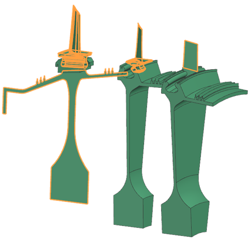
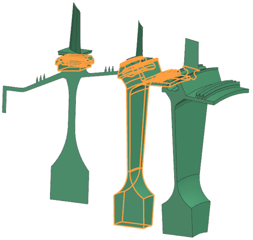
    Axisymmetry Association Zone = Axisymmetric_1 Axisymmetry Association Zone = Axisymmetric_2
  10. Choose Home > Loads and Conditions > Simulation Objects > Source Model Mapping to align models using at least three node pairs.
  11. In the Source Model group, browse to the XML file of the source1 solution which was solved earlier, and click Align Source Model .
  12. Set the Alignment Method to Pairing.
  13. Add at least 3 node pairs to align the two models. You may select any nodes for alignment; however, it is recommended to use nodes on the stage 3 2D blade.
    Use CTRL+F or zoom out to find the source and target models.
  14. Select the Preview check box to see the alignment.
  15. Click Add Pair for each set of nodes to save it in the list.
  16. Click Align.


  17. Click OK.
    The solver populates values in the Translation and Rotation fields
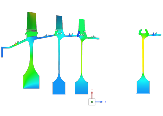
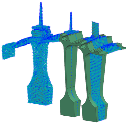
  18. Solve the mapping solution and compare results from the source1 solution.
    Import the results form source1solution.

Create a merged mapping solution

Update the previously mapped solution by replacing the temperatures of disk 2 using results from a second thermal analysis. When creating the merged mapping solution, reference the first Solution 1 mapping solution.

  1. In the Simulation Navigator, right-click Solution 1, select Clone and rename it to Append.
  2. Remove all mapping constraints from the cloned solution but retain the Source Model Mapping simulation object.
  3. Edit the Append solution.
  4. On the Mapping Details page, set the Source Model Results File to the results from the source2 solution, select the Create Merged Result File check box, and reference the results of the first mapping solution.
  5. On the Optional Output page, set the following:
    • Specify a destination directory for the mapping outputs.
    • Select the Nastran check box to generate DAT input files for Nastran.
    • Select the ANSYS check box to generate INP input files for ANSYS.
    • Select the Create ANSYS Solution check box to generate an ANSYS solution within Simcenter 3D.
    • Select the Create Reference Fields for Temperature Loads check box to setup time steps with temperature constraints.
  6. Click OK.
  7. Choose Home > Loads and Conditions > Constraint Type > Mapping Target Set to create a mapping target set limited to disk 2.


  8. Choose Home > Loads and Conditions > Constraint Type > Axisymmetry Target Zone to create an axisymmetric mapping constraint on disk 2, which references the mapping zone in the source model.
  9. Solve the Append solution.
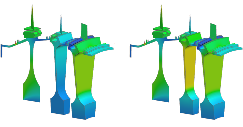
  10. Compare thermal results of each mapping solution and observe the change in the disk 2 temperature.


Inspect generated structural outputs

Review automatically generated solver inputs and reference fields.

  1. Inspect the generated Mapping ANSYS solution.
  2. In one of the solution steps, inspect the Temperature Load and observe that it references a temperature field.
  3. In the Simulation Navigator, under the Fields node, locate this field and confirm in the Field Data Source page, that it directly references the mapping solution BUN file.
  4. Navigate to the output directory and review generated DAT and INP files.
    The ANSYS or Nastran solver directly uses these files. Each file contains a table of Node ID versus Temperature for each time step.

Additional notes

Understand additional mapping options and best practices.

  • Additional output formats for thermal solver and Abaqus are available.
  • If you forget to add a mapping zone in the source model, you do not need to re-solve the solution. Simply add the required mapping constraint to the source model and write the XML input file without running the solve again. The new mapping zones will then appear and can be referenced in the target mapping solution.
  • You can define an angular offset for rotational periodicity mapping constraints. Use this option when the source and target models contain cyclic sectors at different angular positions.