Model a thermal blade root

Model thermal behavior in turbine and compressor blade roots.

Introduction

Thermal modeling of turbine and compressor blade roots represents a common design challenge in gas turbine development. Although you can model these regions in 2D, multiple overlapping thermal boundary conditions often make the approach difficult and less robust.

In this tutorial, you will:

Create 2D/3D and 3D/3D thermal connections.
Create edge and face streams.
Define a duct inlet temperature and connect it to streams.
Connect a duct to a surface using convection.
Define cyclic symmetry on the blade and blade root.

Open and inspect the model

Inspect mesh types, ducts, glue connections, and structural constraints.

Choose File→Open and open blade/GTblade_sim.sim.
In the Simulation Navigator, right-click GTblade_fem.fem and select Make Work Part.
Inspect and confirm the following element types
- The disk uses axisymmetric 2D elements.
- The blade and blade root use 3D elements.
- A 1D duct is defined with the Duct with Mass Flow Axisymmetric properties.
  Use this 1D duct type when modeling cooling networks in gas turbines. It does not require a defined cross-section and expands about the cyclic axis during view factor and convective coupling calculations.
Make the simulation the work part again.
In the Simulation Navigator, under the Face_Glue folder, edit one of the Surface-to-Surface Gluing boundary condition and inspect the settings.

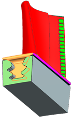
The model uses Surface-to-Surface Gluing with thermal coupling activated. Use glue joints in thermal-mechanical WEM models unless detailed contact behavior at an interface is required. Using a Surface-to-Surface Contact type coupling will cause the structural solver to be much slower. This type of simulation object will model both the thermal and structural connection between the blade and blade root.
Right-click the Face_Glue folder and select Show Only.
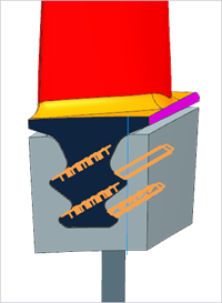
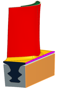
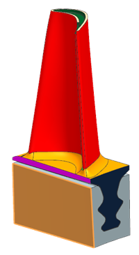
Inspect structural constraints and rotational load.

Apply convective zone and void to the blade

Model external flowpath convection and internal cooling.

Choose Home > Load Type > Thermal Convecting Zone to apply the convective zone to the hot flowpath side of the blade.
Use a convective zone because the mass flow in the flowpath is generally very high and has very high heat capacity and can be assumed constant. Use tangent face selection.
Select the following 28 faces, using the Tangent Faces selection method.
Set the following parameters:
- Fluid Materials = Air
- Temperature = 850 °C
- Pressure = 0.1 MPa
- Heat Transfer Coefficient = 300 W/m² °C
Choose Home > Load Type > Thermal Void to model internal cooling air on the blade.
Modeling the internal cooling passages with a duct network or face streams would provide higher accuracy. However, for this example, a simplified approach is used to estimate blade temperatures. It is assumed that all surfaces for internal cooling convect to the same fluid temperature.
For the region, select the Tangent Faces selection method and click the shown face.
716 faces are selected.
Enter a dummy pressure value for now. You will update a power term once the streams are defined.
Set the heat transfer coefficient to 100 W/m² °C), heat load to 0 W, and select air as a fluid material.
Show only the created void.

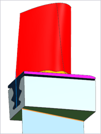
Apply Cyclic Symmetry to 3D components

Define cyclic symmetry on blade and blade root.

Choose Home > Loads and Conditions > Simulation Object Type > Cyclic Symmetry to create a cyclic symmetry object using the cut faces of the blade root.
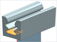
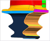
Select the shown face as a source region.
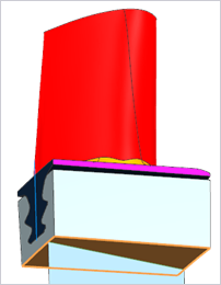
Select the opposite side as a target region.
Click Calculate Segment.
In the Stages group, select the shown bodies.
Set Stage Number (STAGE) to 1.

Note:
When using this approach, ensure the mass flows applied reflect the mass flow of all blades. Convective areas will be scaled appropriately based on the definition of cyclic symmetry.

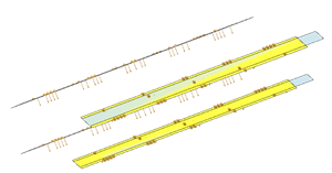
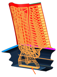
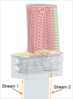
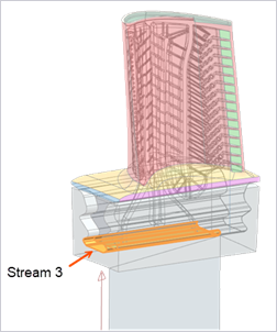
Apply thermal streams

Define radial and axial cooling air streams along the blade root.

The main flow feeds upward into the blade, while a portion of the air leaks through surrounding regions. The following overview describes the streams you will create:


Stream description	Stream illustration
Stream 1 and Stream 2 supply cooling air to the blade with mass flows of 2 kg/s and 0.3 kg/s, respectively.
Stream 3 carries 90% of the flow from Stream 1 into the blade.
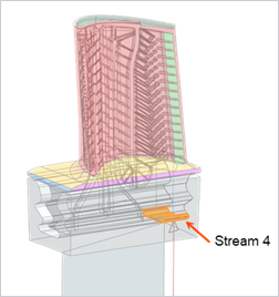
Stream 4 represents leakage from the blade and carries 5% of the flow from Stream 3.
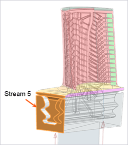
Stream 5 represents a portion of the flow from Stream 1 that bypasses the main path.
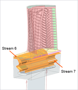
Stream 6 and Stream 7 represent air flowing along the blade, supplied by Stream 5.

Note:

Use Air as the fluid material for all defined streams.

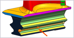
In the Name field, enter Stream%%ID to automatically insert the boundary condition ID into the stream name. This convention helps track stream IDs and verify references throughout the model.

Choose Home > Load Type > Thermal Stream to apply a one-sided edge stream.
The main flow feeds upward into the blade.
Select the shown edge.
Set the following parameters:
- Mass Flow = 2 kg/s
- Inlet Temperature = 300 °C
- Absolute Pressure = 0.1 MPa
- Heat Transfer Coefficient = 200 W/m² °C
Create the second one-sided edge stream on the opposite side with the following parameters:
- Mass Flow = 0.3 kg/s
- Inlet Temperature = 325 °C
- Absolute Pressure = 0.1 MPa
- Heat Transfer Coefficient = 200 W/m² °C
Make sure that the flow direction matches the direction defined in Stream1.
Create the third Two-Sided Stream on Faces.
For the Region - Side A, select the shown 7 faces.
For the Region - Side B, select the shown 5 faces.
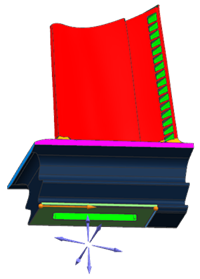
Specify the shown vector by selecting two points.
Set the following parameters:
- Mass Flow = 0.9*smo(1) kg/s
- Inlet Temperature = sto(1)°C
- Absolute Pressure = sp(1) MPa
- Heat Transfer Coefficient = 200 W/m² °C
Create the forth two-sided stream on faces.
For the Region - Side A, select 7 faces.
For the Region - Side B, select 7 faces.
Set the vector as follows.
Set the following parameters:
- Mass Flow = 0.05*smo(3) kg/s
- Inlet Temperature = sto(3)°C
- Absolute Pressure = sp(3) MPa
- Heat Transfer Coefficient = 50 W/m² °C
Create the fifth stream with the Two-Sided Stream on Faces (Cylindrical Components) type.
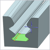
For the Region - Side A, select the shown face.
For the Region - Side B, select 4 faces.
Set the following parameters:
- Mass Flow = smo(1)-smo(3) kg/s
- Inlet Temperature = sto(1)°C
- Absolute Pressure = sp(1) MPa
- Heat Transfer Coefficient = 30 W/m² °C
Note:
In this example, the stream is applied in the radial direction based on the cyclic axis. With a standard stream, the face stream would be applied in the Y direction. In most cases, the difference between these approaches is small, but it may become more noticeable when using larger cyclic sectors.
Create the sixth two-sided stream on faces.
For the region A, select 8 faces.
For the region B, select 7 faces.
Set the vector, as follows:
Set the following parameters:
- Mass Flow = smo(5)/2 kg/s
- Inlet Temperature = sto(5)°C
- Absolute Pressure = sp(5) MPa
- Heat Transfer Coefficient = 50 W/m² °C
For the seventh, repeat the same process as for the Stream6, but for the opposite side.

Note:
The streams that model air flowing along the blade root must be defined separately. If you combine them, the solver may misinterpret interactions between opposing surface normals, since the surfaces can “see” each other. To ensure robust thermal coupling, define separate streams for each region—for example, one stream per region.

Define duct boundary conditions

Define inlet temperature and mass flow for duct and connect to surfaces. Assume that the duct flows radially outward in the Y direction. Define the inlet temperature using a mix function that references the outlet temperatures and mass flows of all streams feeding into this location.

In the Simulation Navigator, display the 1D mesh.
Choose Home > Loads and Conditions > Constraint Type > Temperature to create a temperature constraint on the duct fluid node at the inlet.
In the Region group, from the Selection Method list, select Duct Fluid Nodes.
Set the Type Filter to Node and select the following node.
In the Temperature box, type mix(2,4,6,7) °C.
Choose Home > Loads and Conditions > Simulation Object Type > Duct Flow Boundary Conditions to apply mass flow to the duct using previously defined stream mass flows.
Make sure that the Duct Fan/Pump type is selected.
Select the duct.
In the Mass Flow (per Element), enter smo(6)+smo(7)+smo(4) kg/s.
Choose Home > Loads and Conditions > Simulation Object Type > Thermal Coupling – Convection to create a thermal coupling between duct and surfaces.
Use this approach as an alternative to defining two face streams in this region. You can also apply total temperature effects within the thermal coupling convection definition.
Select the following 2 faces as a Convecting Region.
In the Fluid Ducts, select the duct.
Set the Heat Transfer Coefficient to 50 W/m²°C.

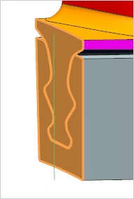
Modify thermal void and apply thermal coupling between disk and root

Update void region and connect disk to blade root thermally.

In the Simulation Navigator, right-click the V1 thermal void and select Edit to modify pressure and power inputs based on your stream ID passing underneath the blade.
Modify the region pressure to sp(3) MPa and heat load to prw(3) W.
Choose Home > Loads and Conditions > Simulation Object Type > Thermal Coupling to create a thermal coupling between the axisymmetric disk and cyclic symmetric blade root.
Select the shown edge as a primary region.
Select the shown face as a secondary region.
Set the Heat Transfer Coefficient to 100000 W/m²°C.

Solve the model and inspect results

Inspect thermal connections and metal temperatures.

Solve the solution.
Display thermal connections.
Inspect the thermal connections to verify that the model establishes connections at all thermal and convective coupling locations. Enable the display of 1D elements if necessary to visualize the contour. Note that the contour key reflects integer values which correspond to different boundary conditions.

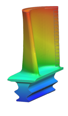
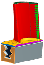
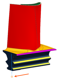
Display metal temperatures for the last increment.

Observe that the blade reaches a higher temperature than the blade root. The metal temperature should remain continuous across the blade root–disk interface, as a very high HTC is defined at that connection.