Using fields to define boundary conditions
Practice the workflow for using formula and table fields to define boundary conditions.
Open the model Simulation file
Open the model Simulation file and reset the dialog box settings.
- Choose File→Open and open field_manifold/ExManifold_sim2.sim.
-
Choose
File→Preferences→User
Interface, on the Dialog and
Precision page, click Reset Dialog
Memory
 .
.
- Click OK.
Create a cylindrical coordinate system
Set up a cylindrical coordinate system to apply thermal constraints.
- In the Simulation Navigator, right-click CSYS and choose New CSYS.
- From the Type list, choose X-Axis, Y-axis, Origin.
- In the Origin Point group, click Point Dialog.
- In the Output Coordinates group, enter the following coordinates: XC: 198.00 mm, YC: 72.25 mm, ZC: 120.00 mm.
- Click OK.
- In the X-axis group, from the Specify Vector list,choose ZC-axis.
- In the Y-axis group, from the Specify Vector list, choose YC-axis.
- In the Settings group, from the Output CSYS list, choose Cylindrical.
- Click OK.
Create a temperature constraint
Apply a spatially varying temperature constraint to the internal surfaces of the exhaust manifold. The mathematical expression representing the temperature variation is written in terms of the cylindrical coordinate system that you created in the previous step. Because all the internal surfaces of interest transition smoothly into one another, you can efficiently select them using the Tangent Faces selection method option.
-
Choose Home tab→Loads and Conditions group→Constraint Type list→Temperature
 .
.
- On the Top Border bar, from Type Filter, select Polygon Face.
- On the scene toolbar, from the Method list, choose Tangent Faces.
-
In the graphics window, select one inner face of the part.
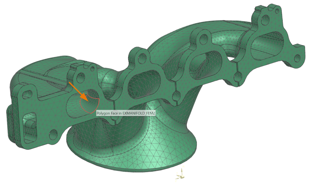
202 faces are selected. -
Next to the Temperature box, click
 and choose New Field → Formula.
- On the Independent Domain tab, from the Independent list, select Cylindrical .
- From the Type list, choose Cylindrical.
- In the Simulation Navigator, expand the CSYS node and click 1-csys to select the created CSYS.
- On the Definition tab, select the temperature row in the table.
- In the box below the table, enter formula: 150 * (1 + cos(theta)) + 300 - abs((z / 1[mm]) - 45).
-
Click Accept Edit
 .
.
-
Click OK in all dialogs.
Display the field to verify that the field is correct.
- In the Simulation Navigator, expand the Fields node.
- Right-click Temperature and choose Plot(XY).
- From the Variable list, select theta.
-
In the Bounds group, in the Minimum box, type 0 and in the Maximum box, type 100.
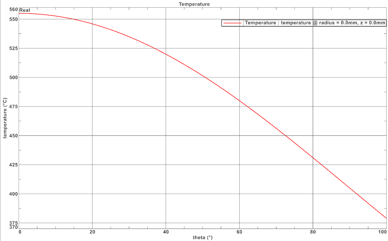
- Click OK and select the graphics window to display the plot.
- Close the graphics window.
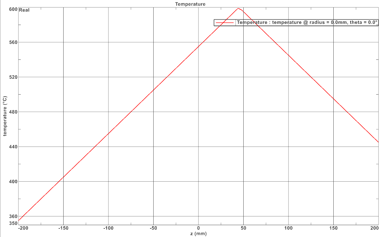
- In the Simulation Navigator, right-click Temperature and choose Plot(XY).
- In the Variable list, select z.
- In the Bounds group, enter a Minimum value of -200 and a Maximum value of 200.
-
Click OK and select the graphics window to display the plot.
Define convection to environment
Define convection constraints with temperature-dependent expression.
- In the Simulation Navigator, expand Constraint Container, right-click Convection to Environment and select Edit.
- In Convection Coefficient box, enter (350-temperature/1[K])*0.001.
- Click OK.
Solve the thermal model
Solve the model and monitor its completion status.
- Right-click Solution 1 in Simulation Navigator and choose Solve.
- Click OK.
- Wait until Complete is displayed in Analysis Job Monitor.
- In the Review Results dialog, click No.
- Close the Information window.
- Click Cancel in Analysis Job Monitor dialog.
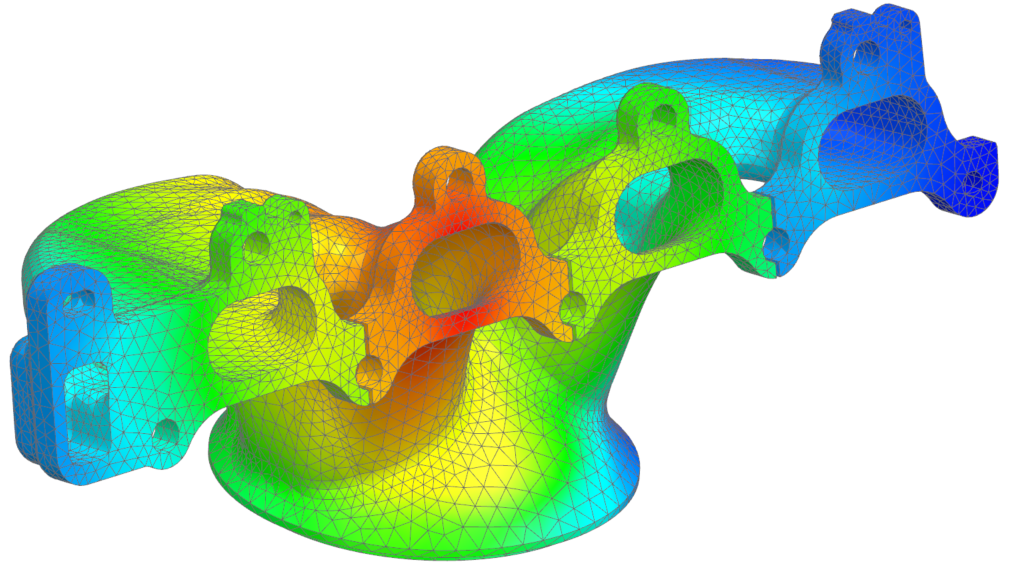
Display the thermal analysis results
Load and review temperature results.
- In the Post Processing Navigator, under Solution 1, right-click Thermal and choose Load.
-
Expand the Thermal node and double-click
Temperature - Nodal.
Create a field from the results
Create a nodal temperature table field from analysis results.
-
Choose Results tab → Tools group → Identify Results
 .
.
- From the Pick list, choose Box(All).
- Drag a box around the result display to select all results.
-
Click Create Field
 .
.
- Click OK.
- Close the Identify dialog box.
-
Choose Results tab → Context group → Return to Model
 .
.
-
In the Simulation Navigator, expand the Fields node, right-click the Nodal Temperature Table field and select Edit.
Observe the created table.