Post process transient results
Practice managing model results using a results probe and graphs.
Open the Simulation file
Open the part file and reset the dialog box settings.
- Choose File→Open and open circuit/circuit_sim1.sim.
- Choose File→Preferences→User Interface.
-
On the Dialog and Precision page, click
Reset Dialog Memory
 .
.
- Click OK.
Visualize the nodal temperature results
Load and explore temperature results.
- In the Post Processing Navigator, right-click the Thermal-Flow node and choose Load.
- Expand the Thermal-Flow→Increment 14, 60.00s nodes and double-click the Temperature-Nodal node.
- Under the Viewports node, expand the Post View 1→asm_pcb1_x_t_fem1.fem→2D Elements→CPU collector nodes and hide CPU mesh.
-
Choose Results tab→Display
group→Edge Style
list→Feature
 to hide the mesh in the post
view.
to hide the mesh in the post
view.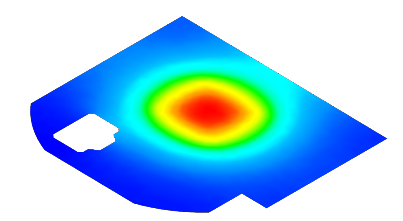
Display the tags for maximum and minimum values
Show annotations for max and min temperature locations and values.
- Under the Post View 1 node, show Annotations.
- Observe the location and value of the maximum and minimum nodal temperature.
Identify results from the model
Select nodes to view their temperature and explore dialog options.
-
Choose Results tab→Tools
group→Identify Results
 .
.
-
Select several nodes from the model to identify their temperature.
The temperature values of the nodes are displayed on the selected item in the graphics window and are also listed in the dialog box.
-
Explore the options in the dialog box.

- Click Close.
-
Choose Results tab→Context
group→Return to Model
 .
.
Create the result variable for the nodal temperature
Define a temperature result variable averaged over nodes.
-
Choose Results
tab→Manipulation group→Result
Variables
 .
.
- Click Create New Variable.
- In the Name box, type Temp.
- From the Result Type list, select Temperature.
- Make sure that Location is set to Nodal and Component is set to Scalar.
- In the Result Combination group, from the Combine At list, select Elements.
-
Make sure that the Criterion is set to Average.
This option controls whether results are averaged across nodes in your model. MIDs (material properties), PIDs (physical properties), and Element Types are selected by default.
- Click OK.
- Click Close.
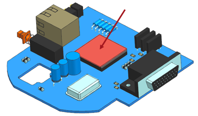
Create a result probe representing the average nodal temperature of the CPU
Create a result probe for the CPU temperature averaged over selected faces.
-
Choose Results tab→Manipulation group→Result Probe
 .
.
- In the Name box, type CPU.
-
In the Formula box, type Temp.
In the formula, Temp is the result variable that you defined in the previous step.
- In the Iteration Definition group, from the Load Case list, select All.
- From the Iteration Selection list, select All.
- Make sure that the Iteration Type is set to Time.
- In the Selection and Averaging group, from the Selection Type list, select Faces.
-
Click Select Object (0)
 .
.
-
In the graphics window, select the CPU top face.
- Select the Compute On Individual Geometry check box to let the software compute a single value on individual geometry.
- From the Geometry Value list, make sure Arithmetic Mean is selected to calculate the average value of all results on the selected geometry.
-
Click Apply.
Do not close the dialog box.
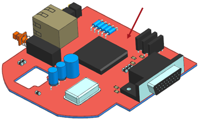
Create a result probe representing the average nodal temperature of the PCB
Create a result probe for the PCB temperature averaged over selected faces.
- In the Name box, type PCB.
- In the Formula box, type Temp.
-
Make sure that the following is selected:
- Load Case = All
- Iteration Selection = All
- Iteration Type = Time
- Selection Type = Faces
-
In the graphics window, select the PCB top face.
-
Click Apply.
Do not close the dialog box.
Create a result probe to evaluate the temperature difference between the CPU and the PCB
Define a result probe for the temperature difference over time.
- In the Name box, type deltaT.
-
In the Formula box, type
fd("CPU")-fd("PCB").
In the formula, CPU and PCB are the result probes that you created in the previous steps. The CPU and PCB fields represent the average nodal temperatures of the CPU and the PCB, respectively.
- In the Selection and Averaging group, from the Selection Type list, select None.
-
Click OK.
Result probe deltaT defines how the difference between the average nodal temperatures of the CPU and the PCB varies as a function of time.
Plot the temperature difference versus time
Plot a graph of the temperature difference over time.
- In the Simulation Navigator, expand the transient → Result Probes nodes.
-
Right-click the deltaT node and choose Create Graph.
Note that the pop-up window is appeared.
-
Click Create a New Window to Plot
 to plot the graph in a separate
window.
to plot the graph in a separate
window.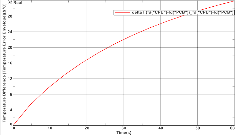
Edit the graph
Modify graph display options and title.
- In the graph window, expand Toolbar.
-
From the Complex Option drop-down list, click
Show and Hide
 .
.
- In the Title row, click Show.
- Click Close to close the Show and Hide dialog box.
- Double-click the title on the graph to modify it.
- In the Text group, click User Defined.
- Modify the text to Temperature difference between the CPU and the PCB.
-
Click OK.

- Explore the other options that you can modify by double-clicking the options on the graph.