Create duct boundary conditions in a thermal model
Practice defining duct boundary conditions in a thermal model. You will specify immersed ducts boundaries and solve a transient solution, using a mold cooling model.
Open the Simulation file
Open the Simulation file and reset the dialog box settings.
- Choose File→Open and open mold_cooling\drone_mold_sim.sim.
- Choose File→Preferences→User Interface and on the Dialog and Precision page, reset the dialog box memory.
Define duct flow boundary conditions
Define inlet and outlet boundary conditions on the ducts.
-
Choose Home tab→Loads and
Conditions group→Simulation Object
Type list→Duct Flow Boundary
Conditions
 .
.
- On the Top Border bar, from the Type Filter list, select Element.
-
In the graphics window, select the displayed element.
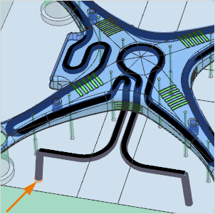
- In the Parameters group, from the Mode list, select Mass Flow.
- In the Mass Flow (per Element) box, type 0.01 kg/s.
- Click Apply.
- From the type list, select Duct Opening.
- On the Top Border bar, from the Type Filter list, select Node.
-
In the graphics window, select the displayed node at the bottom of the
duct.
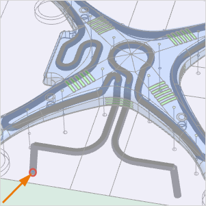
- In the External Conditions group, from the External Temperature list, select Specify.
- In the Temperature Value box, type 20 °C.
- Click Apply.
-
In the graphics window, select the displayed node on the other end of the
duct.
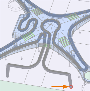
- Click OK.
Define immersed duct boundary condition
Define an immersed ducts boundary condition and specify an expression for the heat transfer coefficient.
-
Choose Home tab→Loads and
Conditions group→Simulation Object
Type list→Immersed Ducts
 .
.
- On the Top Border bar, from the Type Filter list, select Mesh.
-
In the graphics window, select the three displayed meshes representing the
ducts.
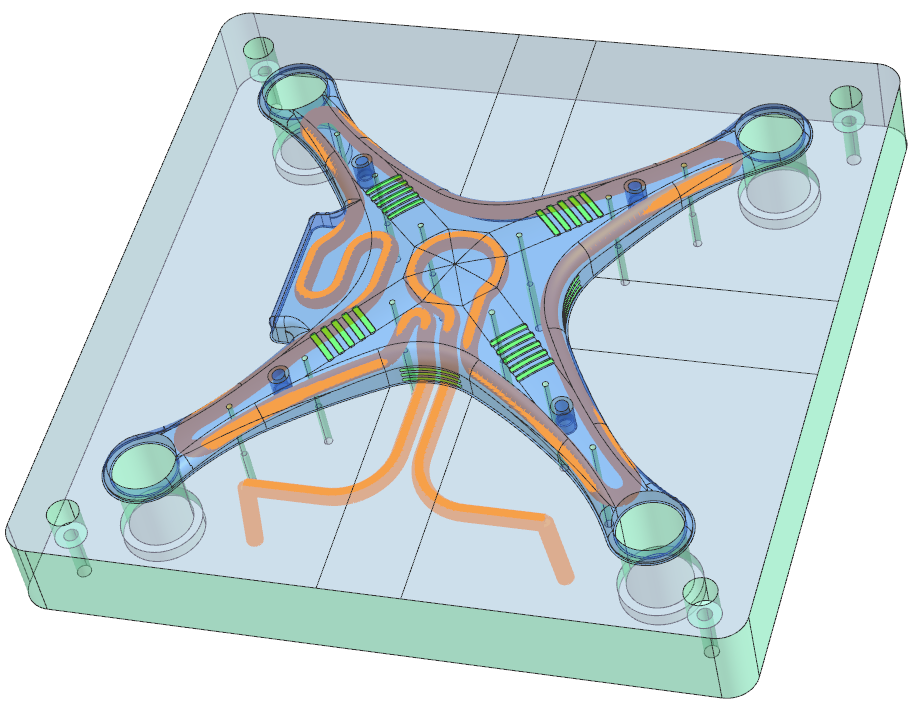
-
In the Magnitude group, in the Heat
Transfer Coefficient box, type 2*HTCFORCE(
2.5,"DUCT_FULL") W/(mm2·°C).
HTCFORCE returns the heat transfer coefficient. DUCT_FULL models the convective heat transfer between the fluid in the duct network, with fully developed flow, and the walls of the duct.
- Click OK.
Solve the model
- In the Simulation Navigator, right-click the Solution 1 node and choose Solve.
- Click OK.
- Wait for the solve to end, before proceeding.
- In the Review Results dialog box, click No.
- Close the Information window.
- In the Analysis Job Monitor dialog box, click Cancel.
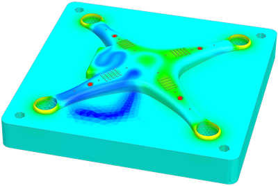
Post process the results
- In the Simulation Navigator, expand the Solution 1→Results nodes and double-click the Thermal node.
-
In the Post Processing Navigator, expand the Thermal→Increment 11, 10.00s nodes, and double-click the Temperature - Elemental node.
-
Choose Results tab→Animation
group→Animate
 .
.
- From the Animate list, select Iterations.
-
Click Play
 to show how the temperature
varies during iterations, and click Stop
to show how the temperature
varies during iterations, and click Stop
 .
.
- Click Close.
- Expand the Post View 1 → Mesh Collectors nodes and hide drone_mold_fem.fem to hide the corresponding meshes.
- Show Annotations to display the maximum and minimum temperature values calculated on the shell elements.
- In the Simulation Navigator, right-click the Solution 1 node, and choose Browse to open the solution directory.
-
Open the drone_mold_sim-Solution_1.GroupReport.htm file to explore the temperature values in each time step.
The solver generates this temperature report over the mold as requested in the drone_report simulation object.
- Compare the mold's maximum and minimum temperature values from the report with those displayed in the graphics window.
- In the Post Processing Navigator, expand the Post View 1→Groups nodes and double-click the Immersed Ducts(1)-Elemental node to identify if the immersed ducts and solid elements are correctly thermally connected.