Apply boundary conditions and solve a satellite model
This is an objective-based lab. Instead of being provided a list of instructions, you are simply provided a scenario and problem statement to solve. Please work to solve the scenario of each activity listed below.
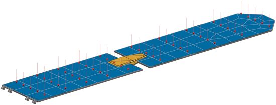
Scenario: You are given a satellite assembly Simulation file, which contains predefined boundary conditions, such as thermal couplings, radiation requests, reports, and thermal heat loads on instruments. You are asked to add boundary conditions for solar panels where necessary. You will create a new Simulation file for the solar panel to define boundary conditions between its parts, import solar panel simulation entities to the satellite assembly Simulation file, define orbital heating and temperature reports, solve the thermal analysis, and post-process the results.
Questions: How to visualize transient temperature results on orbit?
Instructions:
- In the satellite_assembly_bc folder, open solar_panel_fem1.fem.
- Create a new simulation using the Simcenter 3D Space Systems Thermal template for the solar panel to define boundary conditions between the different parts of one solar panel. You do not need to create a solution because the solution, which you will solve, you will create in the HESSI_Satellite_sim1.sim assembly Simulation file.
-
Define a negative heat load of -150W on the bottom layer of solar panel that
represents the power draw.
-
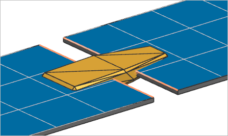
Define an edge contact thermal coupling between the two polygon edges with
conductance per length of 10 W/(m·°C) to represent the middle joint.
Tip: For easier selection, use the Polygon Edge filter type.
- Open the HESSI_Satellite_sim1.sim assembly Simulation file and explore the predefined boundary conditions.
- Import simulation entities, which you created in the solar panel Simulation file, for all instances of the solar panel FEMs by right-clicking the solar_panelfem1.femx4 node and selecting Import Simulation Entities.
-
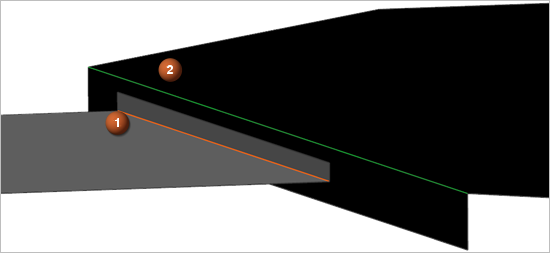
Add edge contact thermal couplings between each solar panel (1) and the main
deck (2) with conductance per length of 5 W/(m·°C).
Tip: For the main deck selection, use QuickPick and make sure that you selected Polygon Edge in FRAME_STRUCT_FEM1.
- Select all created thermal couplings and drag them into the Thermal couplings folder.
- Add solar panel meshes to the selected predefined Top External Radiation group, that is used in the radiation request by right-clicking the group and selecting Add to Group.
-
Create a transient solution with:
- Initial temperature from the steady state solution and transient thermal loads average over the time.
- End time based on orbit period.
- Periodic convergence enabled.
- Implicit integration method with 100 time steps.
- Result sampling of 26 times per orbit. You will use the same value when defining the Hessi orbit.
- Results for last orbit only.
- Request incident fluxes results.
- Add predefined boundary conditions to the solution.
-
Define an orbital heating with the Illuminate Selected
Elements type with predefined Top External
Radiation group in the Top Side Illuminated
Region, bottom solar panels in the Bottom Side
Illuminated Region and the following classical Hessi orbit
modeling object:
- For spacecraft orientation, the first vector aims at Sun and the second
vector aligns with Earth's North as shown.
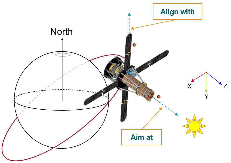
- For the Sun planet characteristics, compute the solar flux for June solstice Sun position.
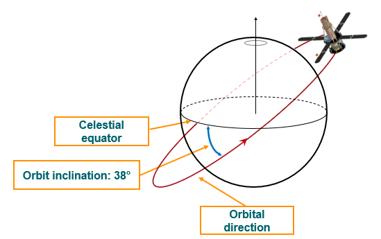
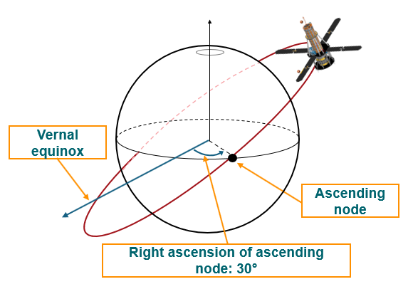
- For the orbit parameters, specify:
Minimum altitude: 600 km Orbit inclination: 38° Satellite position: 30° right ascension of ascending node 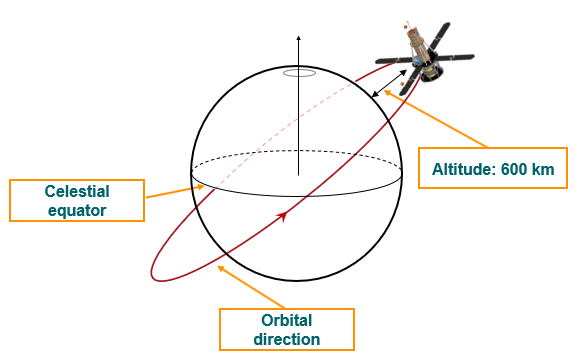
- Specify 26 intervals for the calculation of the satellite positions in the orbit. Greater this number, longer it takes to solve the solution.
- For spacecraft orientation, the first vector aims at Sun and the second
vector aligns with Earth's North as shown.
- Visualize the orbit using the Orbit Visualizer command.
-
Define a temperature report per region for the solar panels top and bottom
layers.
Tip: Use the Solar Panels as a group reference.
- Solve the solution. With the parameters specified, the solution takes around 17 minutes to solve, or import the HESSI_Satellite_sim1-Solution_1.bun file with the results.
-
Post process the results:
- Incident and absorbed fluxes are computed only for the first orbit because they are the same for all orbits.
- Temperature and heat fluxes are displayed only for the last orbit as requested previously.
- Examine the incident solar flux. It is constant except during eclipse.
- Examine the absorbed solar flux.
- Examine the incident planet flux. Animate it to see the changing orientation of the satellite with respect to the planet.
- Examine the temperature. Animate it to see how it varies with time.
- Explore the temperature report by opening the HESSI_on-orbit_600km_NXspace_sim1-Solution_1.GroupReport.htm file in the file directory.
The thermal model is now solved. You will map the temperature result of the source model to the structural target model in the next lab.