Model thermo-optical property degradation
Practice modeling thermo-optical property degradation of the Space Station Remote Manipulator System (SSRMS) by creating thermo-optical state properties, overriding thermo-optical properties in the assembly, and creating multiple solutions for different states of life.
Open the FEM file
Open the FEM file and reset the dialog box settings
- Choose File→Open and open canadarm/ssrms_assyfem1.afm file.
-
Choose File→Preferences→User Interface and on the Dialog and Precision page, reset the dialog box memory.
The SSRMS operates in a low Earth orbit and completes a full orbit in approximately 90 minutes, experiencing solar heating and cold conditions in Earth's shadow which degrade its thermo-optical properties over time.
Create advanced thermo-optical properties
The SSRMS operates in a low Earth orbit and completes a full orbit in approximately 90 minutes. As a result, it is subjected to the intensity of direct solar heating over part of its orbit, followed by the cold conditions in the Earth’s shadow, which degrades its thermo-optical properties over time. You will create three thermo-optical properties: one for beginning of life (BOL), one for middle of life (MOL), and one for end of life (EOL) and one which states point to the previous one. You will use them in three separate solutions that simulate the thermal analysis of the SSRMS in three different times of its useful life.
-
Choose Home tab→Properties
group→More list→Modeling
Objects
 .
.
- In the Create group, from the Type list, select Thermo-Optical Properties - Advanced.
- In the Name box, type BOL and click Create.
- In the Infrared Properties group, in the Emissivity box, type 0.6.
- In the Solar Properties group, in the Absorptivity box, type 0.2 and click OK.
-
Repeat the steps for MOL and EOL properties with emissivity and absorptivity values:
Name MOL EOL Emissivity 0.7 0.8 Absorptivity 0.6 0.8 - In the Simulation Navigator, expand the Modeling Objects node to verify that the three thermo-optical properties are displayed.
- In the Modeling Objects Manager dialog box, in the Create group, from the Type list, select Thermo-Optical Properties - State and click Create.
- In the States group, from the State 1 list,select BOL.
- From the State 2 list, select EOL and from the State 3 list,select MOL.
- Click OK and Close.
- In the Simulation Navigator, under the Modeling Objects node, verify that the Thermo-Optical Properties - State node is displayed.
Override thermo-optical properties
Override the thermo-optical properties and assign the thermo-optical state modeling object to the top radiation settings for mesh collectors, of each component in the assembly. You will modify eleven 2D mesh collectors.
- In the Simulation Navigator, right-click all assembly and FEM nodes with suffix x 2 and choose Unpack.
- In the Simulation Navigator, expand the grapple_fixture_fem1.fem→2D Collectors, right-click Shell(1), select Edit Attribute Overrides.
- In the Thermo-Optical Properties group, in the Top row click No Override and select Apply Override from the Top list, select Thermo-Optical Properties - State1 and click OK.
-
Repeat these steps for all 2D mesh collectors of all FEM in the assembly
and sub-assemblies.
There are 10 additional mesh collectors that you need to override. Notice, that the status of overridden mesh collectors is changed to Applied Override.
- Choose File → Save.
Create a simulation file for the assembly FEM
- In the Simulation Navigator, right-click ssrms_assyfem1.afm and choose New Simulation.
- From the Templates list, select Simcenter 3D Space Systems Thermal.
- In the New File Name group, click Browse and select the canadarm folder.
- Click OK twice.
- In the Solution group, in the Name box, type Solution BOL.
- Click Create Solution
- On the Solution Details page, in the Solve Options group, from the Run Directory list, select Solution Name.
- Click OK.
Define surface-to-surface contact boundary conditions
Create surface-to-surface contacts using automatic face detection.
-
Choose Home tab→Loads and
Conditions group→Simulation Object
Type list→Surface-to-Surface Contact
 .
.
- From the type list, make sure that Automatic Pairing is selected.
-
In the Automatic Face Pair Creation group, click
Create Face Pairs
 .
.
-
In the Create Automatic Face Pairs dialog box, click
OK.
19 face pairs are automatically selected.
- In the Thermal Magnitude group, from the Type list, select Specify.
- From the Conduction Type list, select Heat Transfer Coefficient.
- In the Coefficient box, type 1000 W/(m2°C).
- From the Temperature Dependence Uses list, select Primary Temperature.
- Click OK.
- In the Simulation Navigator, expand the Simulation Objects node, and verify that10 face contact simulation objects are defined.
Define radiation enclosure
-
Choose Home tab→Loads and
Conditions group→Simulation Object
Type list→Radiation
 .
.
- From the type list, select All Radiation type.
- In the Parameters group, from the Element Subdivision list, select 1.
- Click OK.
Define orbital heating
-
Choose Home tab→Loads and
Conditions group→Simulation Object
Type list→Orbital Heating
 .
.
- From the type list, select Illuminate All Elements type.
- In the Name group box, type Orbital Heating ISS.
- In the Orbit Selection group, from the Orbit and Attitude Parameters list, select ISS Orbit.
- In the Parameters group, from the Element Subdivision list, select 1.
- Click OK.
Modify solution attributes
Modify the solution attributes for Solution BOL including setting this analysis to run in parallel to shorten the solve time, which can take up to 30 minutes to solve on a single processor.
- In the Simulation Navigator, right-click Solution BOL and choose Edit.
- On the Solution Details page, in the Solution Type group, from the Solution Type list, select Transient.
- On the Initial Conditions page, from the Initial Temperature list, select Uniform.
- In the Temperature Value box, type 0 °C.
- On the Transient Setup page, in the Solution Time Interval group, from the End list, select Based on Orbit Period.
- In the Maximum Number of Orbits box, type 1.
- In the Results Sampling group, from the Results list, select At Specified Times.
-
Copy the following 13 output times from the output_times.txt file in the Output Times box:
0 695.31 1242.48 1261.78 1390.09 2084.39 2778.53 3472.94 4167.89 4661.4 4680.72 4863.32 5558.9 These output times match the orbital calculation times in order to synchronize the temperature and radiation flux calculations.
-
(Optional) Because the analysis of Solution BOL can
take up to 30 minutes to solve on a single processor, you can set up this
analysis to run in parallel to shorten the solve time, as follows:
- On the Solution Details page, in the Parallel Processing group, select Run Solution in Parallel and click Create New File.
- If an MPI registration window appears, type the user name and password from the computer you are working on.
- In the Enable Parallel table, select the
View Factors and
Solvers check boxes.
The status is displayed as Success. If the status is anything other than Success is displayed, follow the instructions in Validation Output.
- In the No. processes for View Factors and No. processes for Solvers, type 4.
- Choose File→Save and save Parallel Configuration File.xml in the canadarm/Solution BOL folder.
- Close the Parallel Configuration File.xml window.
- Click OK.
Clone the solution twice
- In the Simulation Navigator, right-click the Solution BOL node and choose Clone.
- Rename the cloned solution to Solution MOL.
- Right-click the Solution MOL node and choose Edit.
-
On the Thermal page, in the Thermo-Optical Property State box, type 3.
The state number indicates which thermo-optical properties from the Thermo-Optical Properties - State modeling objects referenced in the model the thermal solver uses during the solve.
- Click OK.
- In the Simulation Navigator, right-click the Solution MOL node and choose Clone.
- Rename the cloned solution to Solution EOL.
- Right-click the Solution EOL node and choose Edit.
- On the Thermal page, in the Thermo-Optical Property State box, type 2.
- Click OK.
(Optional) Solve all solutions
You can request that the software solves all three solutions sequentially one after the other. On six processors, each solutions takes approximately 10 minutes to solve, so the total solve time for all three solutions is approximately 30 minutes. You can use these steps to solve the solutions or you can go directly to next section because the solved result files are included in the canadarm folder. The solved result files are included in the canadarm folder.
- In the Simulation Navigator, right-click the ssrms_assyfem1_sim1.sim node and choose Solve All Solutions.
-
In the Solve All Solutions dialog box, clear the
Skip Solutions with Results check box and click
OK.
When you use the Solve All Solutions command, the software is not accessible until the last solution is finished solving. The Solution Monitor shows you the progress of the current solution. The Summary of Solutions dialog box shows the number of solutions selected, skipped, failed, and solved. When the last solution is finished solving, Simcenter 3D becomes responsive again.
- In the Summary of Solve all Solutions dialog box, click OK and close the Information window.
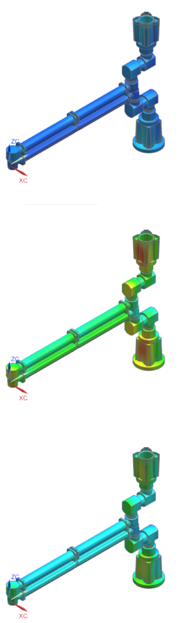
Display results
Load the thermal results for each solution and view results..
- In the Post Processing Navigator, under the Solution BOL, the Solution MOL, and the Solution EOL nodes, select each Thermal node, press Ctrl, right-click the selection and choose Load.
-
Choose Results tab→View
Layout group→Three Landscape Views
 .
.
- In the Post Processing Navigator, under the Solution BOL node, expand the Thermal → Increment 12, 4863.32 s node, double-click the Temperature – Elemental node and, in the graphics window, select the upper viewport.
- Under the Solution MOL node, expand the Thermal → Increment 12, 4863.32 s node, double-click Temperature – Elemental node and, in the graphics window, select the middle viewport.
- Under the Solution EOL node, expand the Thermal → Increment 12, 4863.32 s node, double-click the Temperature – Elemental node and, in the graphics window, select the lower viewport.
- In the Post Processing Navigator, select Post View 1 and press Ctrl, select Post View 2 and select Post View 3.
-
Choose Results tab→Display
group→Edge Style list→
Feature
 .
.
-
Choose Results tab→ Post View
group→ Edit Post View
 .
.
- On the Legend tab, in the Color Bar group, from the Legend Extremes list, select Specified.
-
In the Max box, type
52.
To have the same legend extremes for the three viewports, the minimum value is from the upper viewport (-35.8 °C) and you specify the maximum value to 52 °C, which is the maximum temperature from Solution EOL, the lower viewport.
- Click OK.
-
Choose Results tab→Utilities
group→View Synchronize
 .
.
-
Select all three viewports and click OK.