Model orbital maneuvers of a communication satellite
Practice modeling the orbital maneuvers of a communication satellite to prevent the camera from facing the Sun to avoid overheating and to ensure it turns towards the Earth during eclipses to capture images. You will visualize the defined orbits using the Orbital Visualizer. You will learn how to model orbital heating to simulate the thermal response of a satellite in orbit around Earth.
Open the Simulation file
Open the Simulation file and reset the dialog box settings.
- Choose File→Open and open satellite_orbital/communications_satellite_sim1.sim file.
- Choose File→Preferences→User Interface and on the Dialog and Precision page, reset the dialog box memory.
-
In the Simulation Navigator, explore the following predefined boundary conditions:
- A Radiation simulation object to define the radiative exchange between the satellite and the environment.
- Surface-to-Surface Contact simulation objects defined between the different bodies of the model to specify the thermal contact.
Model the full orbit maneuver
Set all parameters that define a full orbit using the Orbit modeling object.
-
Choose Home tab→Properties
group→Modeling Objects
 .
.
- In the Create group, from the Type list, select Orbit.
- In the Name box, type Full Orbit.
- Click Create.
-
In the Properties group, in the Orbit
Type box, make sure that Classical is
selected.
The classical orbit type allows you to define the maximum allowable orbit parameters.
-
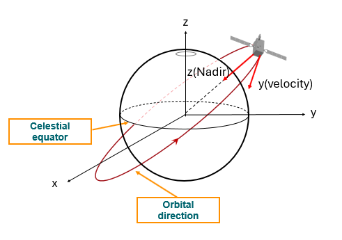
On the Spacecraft Attitude page, in the
Orientation Options group, from the first
Specify Vector list, select the
ZC-axis that aims at Nadir and from the second
Specify Vector list, select the
YC-axis that aligns with the Velocity
Vector as shown.
-
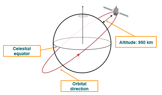
On the Orbit Parameters page, in the
Minimum Altitude box, type 950
km to specify the minimum distance of the orbit from the
Earth's surface.
-
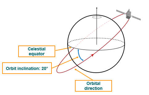
In the Orbit Inclination box, type
20 to specify the orbit inclination angle. This
is the angle between the orbit plane and the equatorial plane, equivalent to
the angle between the planet's axis and the orbit's normal.
- Make sure that the Satellite Position is set to Local Time at Ascending Node which is set to midnight.
- On the Calculation Positions page, in the Orbit Segment group, from the Segment Type list, make sure that Full Orbit is selected.
- Make sure Start Angle Referenced from is set to Ascending Node.
-
In the Intermediate Calculation Positions group, in
the Number of Intervals box, type
8 to set the number of orbit divisions for
calculation points.
The solver calculates black body view factors, solar, earth and albedo view factors and resulting heat loads at each calculation position on the orbit. All calculation positions are referenced from the start angle you select, and the spacecraft position at the beginning of the transient analysis. Regardless of any intermediate calculations you specify, results are always calculated at both the initial position of the spacecraft, and last defined position of the spacecraft. These two calculation positions are respectively 0° and 360° from the start angle for a full orbit.
- Click OK and Close.
Define the orbital heating for the full orbital maneuver
Create the Orbital Heating simulation object and use the Orbit Visualizer to display the full orbit to define the start and end time of eclipse.
-
Choose Home tab→Loads and
Conditions group→Simulation Object
Type→Orbital Heating
 .
.
- Select Illuminate Selected Elements from the list.
- In the Name group, type Orbital Heating (Full Orbit).
- In the Top Side Illuminated Region group, select the Group Reference check box.
- In the table, select External surfaces - TOP group, which contains all the surfaces of the satellite in contact with the environment.
- In the Bottom Side Illuminated Region group, select the Group Reference check box.
- Select External surfaces - BOT group in the table, containing eight surfaces of solar panels.
- In the Orbit Selection group, select Full Orbit from the Orbit and Attitude Parameters list.
-
In the Parameters group, select
Deterministic in the Calculation
Method box.
Notice that the Hemicube Rendering method is not available because it does not support the computation of radiative heat loads and the transmissive and specular thermo-optical properties.
-
In the Parameters group, from the Element
Subdivision list, select 1.
A small element subdivision value will reduce the computational time.
- Click OK.
-
Choose Home tab→Space
group→Orbit Visualizer
to visualize the full orbit
maneuver.
-
In the File Operation, click
Options
 .
.
- Click Default.
-
Select the following check-boxes:
- Calculation Positions to display positions of the satellite.
- Dawn-Dusk Line to display the imaginary line on a planetary body that separates the illuminated day side from the dark night side.
- Shadow Cone to display the zone where the planet hides the sun from the satellite.
- Click Dismiss.
-
Choose View→Normal to Orbit to display the view from normal to orbit.
You can use Zoom to adapt the display to your screen.
-
In Animation, click to display the position of the
orbit at which eclipse starts.
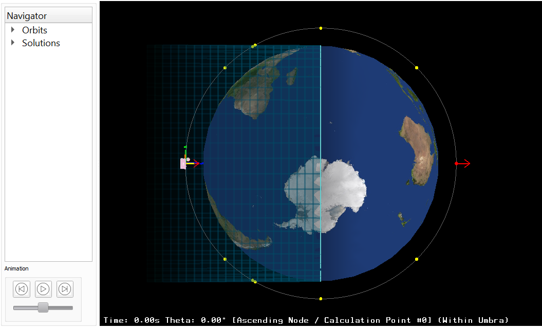
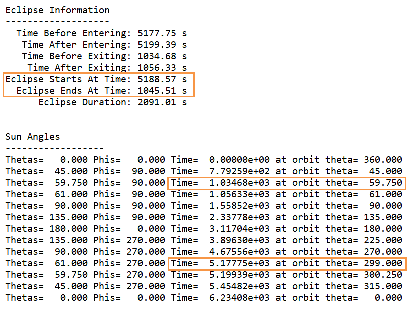
Observe the time and angle of the calculation point. - Display the position of the orbit at which eclipse ends.
-
In the File Operation, click Orbit
Info
 to list the eclipse and sun
angles information.
to list the eclipse and sun
angles information.
- In the Eclipse Information, notice that the eclipse starts at 5188.57 s and ends at 1045.51 s.
-
In the Sun Angles, you can find the angles that
correspond to start and end times, which are 299 and 59.75
respectively.
- Close the Orbit Info window and Orbit Visualizer.
Model the parent orbit maneuver
Define the partial orbit maneuver of the satellite that will start from the end position of the eclipse. In the previous step, we found the start and end angles of the eclipse. Since the maneuver does not start right away, to simplify calculation, we will use 295° and 60° angles.
- In the Simulation Navigator, under the Modeling Objects node, right-click Full Orbit and select Clone.
- In the Name box, type Orbit-Sun.
- On the Sun Planet Characteristics page, in the Planet Data group, in the Prime Meridian Initial Position Referenced from list, select Ascending Node.
- On the Calculation Positions page, in the Orbit Segment group, from the Segment Type list, select Partial Orbit.
- In the Start Angle box, type 60°.
- In the End Angle box, type 295°.
- Click OK.
Model the child orbit maneuver
Define the child orbit maneuver of the satellite that will start from the end position of the Orbit-Sun orbit.
- In the Simulation Navigator, under the Modeling Objects node, right-click Orbit-Sun and select Clone.
- In the Name box, type Orbit-Eclipse.
- On the Spacecraft Attitude page, in the Orientation Options group, from the first Specify Vector list, select the XC-axis that aims at Nadir and from the second Specify Vector list, select the YC-axis that aligns with the Velocity Vector.
- On the Calculation Positions page, in the Orbit Segment group, select the Match Start Time with End of a Parent Orbit check box.
- From the Parent Orbit list, select the Orbit-Sun orbit.
-
Set the orbit segment parameters:
- Angles Referenced from = Ascending Node
- Start Angle = 295°
- End Angle = 360+60°
- In the Intermediate Calculation Positions group, in the Number of Intervals box, type 4.
- Click OK.
Define the orbital heating for the complete orbital maneuver
Create two Orbital Heating simulation objects to model the thermal response of the satellite during the complete orbital scenario.
- In the Simulation Navigator, under the Simulation Object Container node, right-click the Orbital Heating (Full Orbit) node and select Clone.
- In the Name group, type Orbital Heating (Orbit-Sun).
- In the Orbit Selection group, from the Orbit and Attitude Parameters list, select Orbit-Sun.
- Click OK.
- In the Simulation Navigator, under the Simulation Object Container node, right-click the Orbital Heating (Orbit-Sun) node and select Clone.
- In the Name group, type Orbital Heating (Orbit-Eclipse).
- In the Orbit Selection group, from the Orbit and Attitude Parameters list, select Orbit-Eclipse.
- Click OK.
- In the Simulation Navigator, under the Simulation Object Container node, select Orbital Heating (Orbit-Sun) and Orbital Heating (Orbit-Eclipse), right-click and select Add to active solution or step.
- In the Simulation Navigator, under the Solution 1 node, right-click Orbital Heating (Full Orbit) and select Remove.
-
Choose Home tab→Space
group→Orbit Visualizer
.
- In the Navigator, expand Solutions and select Solution 1.
-
In the Animation, click Play
 .
.
- Close the Orbit Visualizer.
Define the transient parameters
- In the Simulation Navigator, right-click the Solution 1 node and choose Edit.
- On the Transient Setup page, from the End list, select Based on Cyclic Criterion to specify the solution end time.
- In the Maximum Number of Cycles box, type 15.
- In the End Solve if Temperature Change Between Cycles less than box, type 0.1.
- In the Specify Cycle Period box, type 8640.
- In the Time Integration Control group, from the Time Step Option list, select Constant.
- In the Time Step box, type 120 s.
- Click OK.
Solve the model
- In the Simulation Navigator, right-click the Solution 1 node and choose Solve.
- Click OK.
- Wait for the solve to end, before proceeding. The solve takes around 10 minutes to complete.
- In the Review Results dialog box, click No.
- Close the Information window.
- In the Analysis Job Monitor dialog box, click Cancel.
Review and animate the results
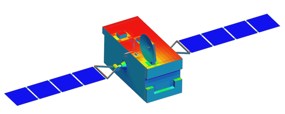
Display the temperature results and animate the results.
- In the Simulation Navigator, double-click the Results node.
- In the Post-Processing Navigator, expand the Thermal → Increment 10, 4.069E+03s nodes, and double-click the Earth View Factor - Elemental node.
-
Choose Results tab→Display
group→Edge Style
list→Features
 .
.
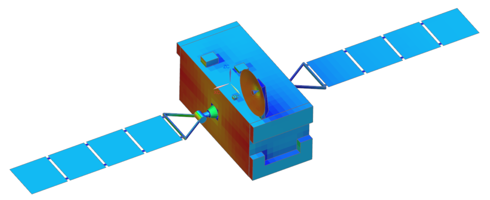
-
In the Post-Processing Navigator, expand the
Thermal → Increment 11,
4.139E+03s nodes, and double-click the Earth View
Factor - Elemental node.
Visualize the results using the Orbit Visualizer
Use the Orbit Visualizer to display the results at every calculation position during the last orbit maneuver. You will visualize the effect of the satellite trajectory on the solar and earth view factors.
-
Choose Results tab→Context
group→Return to Home
 .
.
-
Choose Home tab→Space
group→Orbit Visualizer
.
-
Click Results
 to specify the results BUN file
and the result type used to display the results on the spacecraft orbiting
the planet in the graphics window.
to specify the results BUN file
and the result type used to display the results on the spacecraft orbiting
the planet in the graphics window.
- Next to the Results File box, click Browse to load the communications_satellite_sim1.bun file that contains the results of the simulation.
- From the Select Results Type list, select Earth View Factor-Elemental.
- Click OK.
-
In the File Operation, click
Options
.
- On the Size tab, move the Model Size slider completely to the right to increase the size of the satellite in the Orbit Visualizer graphics window.
- Click Dismiss.
-
In Animation, click Play
.
- Close the Orbit Visualizer.