Model multi-layer shells and thermal protection system
Practice modeling multilayer shells and thermal protection system for a satellite.
Open the Simulation file
Open the Simulation file and reset the dialog box settings.
- Choose File→Open and open satellite_multilayer/communications_satellite_sim1.sim file.
- Choose File→Preferences→User Interface and on the Dialog and Precision page, reset the dialog box memory.
-
In the Simulation Navigator, explore the following predefined boundary conditions:
- A Radiation simulation object to define the radiative exchange between the satellite and the environment.
- A Solar Heating Space simulation object to specify the solar load on the satellite.
- Several Surface-to-Surface Contact simulation objects defined between the different bodies of the model to specify the thermal contact.
Model the thermal protection blanket of the satellite bus using a thin shell property
Modify the 2D mesh collectors of the satellite bus and specify a new thin shell property to model the thermal blanket. You will assign a new material and thermo-optical properties to the 2D mesh collectors.
- In the Simulation Navigator, right-click the communications_satellite_fem1.fem node and choose Make Work Part.
- Expand the communications_satellite_fem1.fem→2D Collectors nodes, right-click the Bus node and choose Edit.
-
In the Material group, click Choose
material
 .
.
-
In the New Material group, click Create
material
 .
.
- In the Name - Description box, type thermal_blanket.
- In the Properties group, in the Mass Density (RHO) box, type 1200 kg/m3.
-
On the Thermal page, in the Thermal group, specify the following properties:
- Thermal Conductivity (K) = 0.024 W/(m·K)
- Specific Heat (CP) = 1674 J/(kg·K)
- Click OK twice.
- In the Physical Property group, from the Thin Shell Property list, select 3mm shell.
- In the Thermo-Optical Properties group, in the Radiation box, make sure that Top is selected to allow only the top face of the bus surface to exchange through radiation.
-
Next to the Top list, click Open
Manager
 .
.
- In the Create group, from the Type list, select Thermo-Optical Properties - Advanced.
- In the Name box, type blanket.
- Click Create.
- In the Properties group, in the Emissivity box, type 0.016.
- In the Absorptivity box, type 0.003.
- Click OK and Close.
- Click OK to close the Mesh Collector dialog box.
Model the solar panels using multi-layer shells non-uniform
Modify the existing 2D mesh collector of the satellite solar panels. You will create a non-uniform multi-layer shell property, containing a stack of four layers with different thermo-optical properties. You will also specify the thermal coupling between the different layers.
- In the Simulation Navigator, under the 2D Collectors node, right-click the Solar Panels node and choose Edit.
- In the Properties group, from the Type list, select Multi-Layer Shell Non-Uniform.
-
Next to the Layer Stack Property list, click
Create Physical
 .
.
- In the Physical Property Table group, in the Name box, type Multi-layer panels.
-
In the Properties group, click Create
Stack Layers (First Layer is Top Layer)
 .
.
- In the Create group, in the Name box, type Top layer, and click Create.
- In the Properties group, from Material list, select Aluminum_6061.
- In the Thickness box, type 1 mm.
- From the Radiation list, select Top to activate the radiation calculation for the top surface of the top layer.
- From the Top list, select Vapor-deposited coating - Silver.
- Click OK.
- In the Create group, in the Name box, type Middle layer_1, and click Create.
- In the Properties group, from Material list, select Aluminum_6061.
- In the Thickness box, type 20 mm.
- From the Radiation list, select None to deactivate the radiation calculation for the middle layer.
- From the Coupling Magnitude list, select Specify.
- In the Account for box, make sure that Conduction is selected to model conduction between the middle layer and the top layer.
- In the Heat Transfer Coefficient box, type 0.5 W/(m2·°C).
- Click OK.
- In the Create group, in the Name box, type Middle layer_2, and click Create.
- In the Properties group, from Material list, select Aluminum_6061.
- In the Thickness box, type 10 mm.
- From the Radiation list, select None to deactivate the radiation calculation for the middle layer.
- From the Coupling Magnitude list, select Specify.
- In the Account for box, make sure that Conduction is selected to model conduction between the middle layer and the top layer.
- In the Heat Transfer Coefficient box, type 0.5 W/(m2·°C).
- Click OK.
- In the Create group, in the Name box, type Bottom layer, and click Create.
- In the Properties group, from Material list, select Aluminum_6061.
- In the Thickness box, type 1 mm.
- From the Radiation list, select Bottom to activate the radiation calculation for the bottom surface of the bottom layer.
-
From the Bottom list, select Solar Cells
- COMSAT.
This modeling object contains the thermo-optical properties of the solar cells used by the COMSAT company in communication satellites.
- From the Coupling Magnitude list, select Specify.
- In the Account for box, make sure that Conduction is selected to model conduction between the bottom layer and the middle layer.
- In the Heat Transfer Coefficient box, type 0.5 W/(m2·°C).
- Click OK.
- In the Selection group, select Top layer, press and hold Ctrl and select Middle layer and Bottom layer.
-
In the List group, click Add
 .
Make sure that the layers are in the following order: Top layer, Middle layer_1, Middle layer_2, Bottom layer. The solver will use this order during the solve.
.
Make sure that the layers are in the following order: Top layer, Middle layer_1, Middle layer_2, Bottom layer. The solver will use this order during the solve. - Click Close and OK for all dialog boxes.
Solve the model
- In the Simulation Navigator, right-click communications_satellite_sim1.sim node and choose Make Work Part.
- Right-click the Solution 1 node and choose Solve.
- Click OK.
- Wait for the solve to end, before proceeding.
- In the Review Results dialog box, click No.
- Close the Information window.
- In the Analysis Job Monitor dialog box, click Cancel.
Review the results
Display the temperature results and review the temperatures of the different layers of the multi-layer shell.
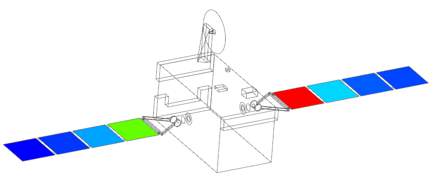
- In the Simulation Navigator, double-click the Results node.
- Expand the Thermal → Increment 25, 4.320E+04s, double-click the Temperature - Elemental node.
-
Choose Results tab→Display
group and from the Edge Style list, select
Features
 .
.
The Ply 1 reports the temperature results at the bottom layer of the multi-layer shell, which has the solar panels properties. Notice that the highest temperatures are on the solar panels surfaces, which face the sun. -
Choose Results tab→Post View
group→Edit Post View
 .
.
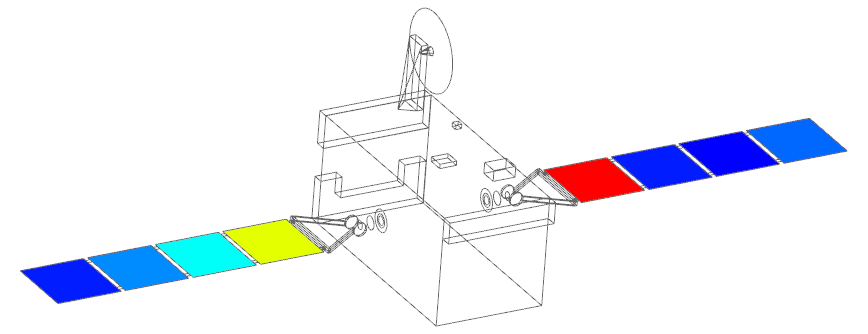
- In the Result Type group, select Ply 4.
-
Click OK.
The Ply 4 reports the temperature results at the top layer of the multi-layer shell, which has a conductive thermal coupling with the middle layer of the multi-layer shell. The temperature is lower than the top layer because this side of the solar panels is not receiving the solar load. -
Choose Results tab→Post View
group→Edit Post View
.
- In the Result Type group, select Ply 3.
-
Click OK.
The Ply 3 reports the temperature results at the middle layer of the multi-layer shell, which has a conductive thermal coupling with the top and bottom layers.