Wall functions
Wall functions describe the flow velocity as a function of distance from the wall within the near-wall region in the turbulent boundary layer. By using wall functions to approximate the mean velocity field in the near-wall region, you avoid mesh requirements needed to resolve the viscous sublayer.
Turbulent boundary layer
The turbulent boundary layer that forms over a flow surface is characterized by the sharp velocity gradient along the direction normal to the wall as shown in the following picture of the velocity profile near a wall.

The turbulent boundary layer is divided into the inner layer (4) and the outer layer (5).
|
Red: mean velocity Blue: mean velocity in viscous sublayer Green: mean velocity in log-law region |
|
The inner layer in turn is divided into:
-
The viscous sublayer (1): y+ < 5
- The buffer layer (2): 5 < y+ < 30
- The log-law region (3): 30 < y+ < 200
Boundary layer meshes, which are high aspect ratio grids with very fine spacing along the wall normal direction, are typically used inside boundary layers in order to capture the sharp velocity gradient while maintaining a reasonable overall grid count and computational efficiency. The appropriate mesh size next to walls is determined by the non-dimension distance value y+ defined as follows:
where:
- For body-fitted fluid meshing, Δy = Δyp is the distance between the centroid (point P) of the wall-adjacent control volume and the wall. You can approximate Δyp from the distance of the first node and the wall, Δye, as Δye/4 ≤ Δyp ≤ Δye/3. In the following graphics, the centroid is represented by the point P.
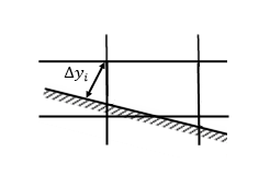
For immersed boundary meshing, Δy = Δye, avg is the average value of the normal wall distances between the boundary element's N nodes and the closest immersed wall boundary.
-
ρ and μ are density and dynamic viscosity of the fluid.
- τw is the wall shear stress.
In the viscous sublayer, the mean velocity represented by the red curve, is given by the following equation represented by the blue curve:
-
where U+ is the dimensionless velocity computed as:
In the log-law region, the mean velocity is given by the log-law equation represented by the green curve:
- where C+ is an experimental constant.
Standard wall function
The standard wall function is represented by the red curve in the graphic: Velocity in the turbulent boundary layer.
The flow solver uses general form of exponential blending function between the linear relation in the viscous sublayer and the classical log-law from the log-law region as follows:
When you request the standard wall function, you should place the first computational nodes above the wall in the log-law region. If the node is located in the viscous sublayer, the results are inaccurate. You can use wall function only for streamlined geometries without flow separation.
Hybrid wall function for K-Omega and SST models
Standard wall function performance deteriorates when the first layer grid is in the buffer layer or viscous sublayer. Hybrid wall function ensures a locally appropriate near-wall resolution adapted to the flow structures and it is robust even when y+ < 30. Hybrid wall function is also more robust, when the flow approaches the separation point.
The hybrid function blends the Reichardt's law FReimix and Spaldings law FSp,3 as follows [36]:
Reichardt's law of the wall is defined as follows:
The following blending is applied with classical log-law:
Spaldings law is given by the following inverse formula:
Hybrid wall function for Spalart-Allmaras model
The hybrid wall function blends Reichardt's law FReimix and Spaldings law FSp,5 as follows [35]:
where:
Reichardt's law of the wall is defined as follows:
The following blending is applied with classical log-law:
where:
Spaldings law is given by the following inverse formula: