1D network connected to 3D fluid region
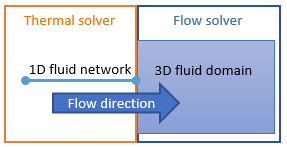
In a coupled thermal-flow analysis, you can couple a 3D fluid domain to a set of thermal streams and ducts with mass flow from a 1D fluid network that has the same fluid material. The flow solver solves the equations on the 3D fluid domain using the information from the 1D fluid network solved by the thermal solver.
Flow Directions
| Fluid flows from 1D network to 3D domain | Fluid flows from 3D domain to 1D network |
|---|---|
 |
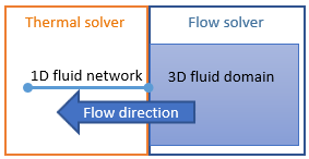 |
When the fluid flows from the 3D domain to the 1D network, you can specify the flow alignment, turbulence characteristics, and define a radially varying swirl in the fluid if your model requires it.
Transfer options between solvers
Irrespective of the flow direction, the thermal solver always transfers the fluid quantities from the 1D fluid network to the 3D fluid domain at the junction. You specify whether the mass flow rate () or pressure (P) is transferred. The flow solver computes the other quantity.
The thermal and the flow solvers exchange the temperature at the junction as the boundary temperature of the other solver.
If the flow direction is from the 3D domain to the 1D network and you request that the thermal solver automatically determines the inlet temperature of the stream, the flow solver transfers the temperature from the 3D flow surface to the inlet of the stream.
Transferring mass flow rate to the 3D fluid domain
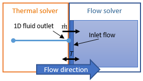
| Fluid flows from 1D network to 3D domain | Fluid flows from 3D domain to 1D network |
|---|---|
 |
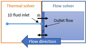 |
| The flow solver treats the selected 2D surface as an inlet flow with mass flow rate value transferred from the junction by the thermal solver, which is the outlet value of the thermal stream or duct. | The flow solver treats the selected 2D surface as an outlet flow with mass flow rate value transferred from the junction by the thermal solver, which is the inlet value of the thermal stream or duct. |
Multiple 1D fluid connections
When transferring mass flow rate, you can connect multiple streams and ducts to the 3D fluid domain at the junction. At each junction, the flow solver controls the mass flow using the conservation of mass equation:
Where:
- is the mass flow rate of a 1D duct or stream
- is the mass flow rate transferred to the 3D fluid domain.
Because the mass flow value of each stream or duct can be positive or negative, the solvers adapt automatically to the direction of the 1D fluid.
Transferring pressure to the 3D fluid domain
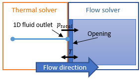
When you specify the pressure transfer, the flow solver always treats the selected 2D surface of the 3D fluid domain as an opening.
| Fluid flows from 1D network to 3D domain | Fluid flows from 3D domain to 1D network |
|---|---|
 |
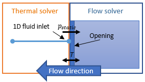 |
| The 1D fluid pressure from the outlet of the stream or duct is specified as the opening total pressure. For more information, see Inflow vent. | The 1D fluid pressure from the inlet of the stream or duct is specified as the opening static pressure. For more information, see Outflow vent. |
The thermal solver allows only one stream or duct to be connected to the 3D fluid domain when a pressure transfer is specified.
You can manually override the pressure value transferred by the thermal solver using an expression, a formula, a table, or a table of fields. For example, this may be useful if you would like to keep a constant pressure value at some locations.