Home
Flow Solver
Contains flow solver related guides, such as the reference and API guides.
Flow solver reference
Insert short description here
Discretization
The following section describes the discretization methods used by the flow solver to discretize the governing equations.
Control-volume method
The flow solver uses a finite-element based control-volume method for discretization of the governing equations. With this method, the governing equations are integrated over a control volume and over a time step.

Flow Solver
Contains flow solver related guides, such as the reference and API guides.
- Flow solver guides
  Maya HTT's flow solver is included and distributed with Simcenter 3D and Simcenter Femap. This page contains links to flow solver guides, which help you understand how the flow solver works.
- Flow solver reference
  Insert short description here
  - Introduction
    The flow solver computes a solution to the non-linear, partial differential equations for the conservation of mass, momentum, energy, and general scalars in general complex 3D geometries. It uses an element-based finite volume method and iterative Krylov methods to discretize and solve the governing equations.
  - Nomenclature
    The nomenclature table offers a description and sample units or constant values of the variables used in the Flow Solver Reference Manual.
  - Governing equations
    A model can be comprised of multiple flow enclosures. Each enclosure is a separate group of three-dimensional elements that form a separate fluid domain from the remaining geometry. The physical scales of each enclosure, such as the length scale, time scale, pressure, and temperature are independent of the other enclosures. The flow solver solves governing equations separately for each flow enclosure.
  - Source term
    The source term can represent body forces or flow resistance forces to model different physical phenomena.
  - Turbulence models
    In the flow solver, the flow field can be solved as laminar or as turbulent using governing equations.
  - Boundary conditions
    This section outlines different boundary conditions supported by the flow solver and the associated considerations.
  - Modeling a gas mixture
    The flow solver uses the scalar equation to model a gas mixed in any proportion with the main gas. The software supports up to five gases in the mixture. All gases are assumed to behave as ideal gases using the ideal gas law.
  - Modeling humidity
    The flow solver uses the gas mixture scalar equation to model humidity that is defined as a mixture of water vapor in air.
  - Modeling non-Newtonian fluid
  - Modeling particle tracking
    The following section describes the equations and forces that model particle trajectories, including treatment and effects of boundary conditions
  - Modeling fluid structure interaction
    Fluid structure interaction (FSI) computations account for motion or deformation of the solid structure boundaries that are interacting with the adjacent fluid flow. The flow solver handles both transient and static fluid structure interactions.
  - Discretization
    The following section describes the discretization methods used by the flow solver to discretize the governing equations.
    - Control-volume method
      The flow solver uses a finite-element based control-volume method for discretization of the governing equations. With this method, the governing equations are integrated over a control volume and over a time step.
    - Spatial discretization
      This section describes the spatial discretization of the governing equations and the terms that compose them.
    - Temporal discretization
      The flow solver uses the Backward Euler and Crank-Nicolson schemes, and the local time step method as time discretization methods.
    - Other discretization methods
      The following section describes discretization methods such as the disjoint mesh pairing method, the immersed boundary, or various mesh moving methods.
  - Solver numerical methods
    The following section describes numerical methods used by the flow solver such as the linear equation solution, which acts as a preconditioning method to the basic iterative algorithm, and other solver methods, such as Krylov methods.
  - Flow solver files
    The following table describes the flow solver files, which are written in the run directory during the solving process.
  - Flow solver bibliography
    The following bibliography lists all sources used to explain how the flow solver works.
- Flow solver flowcharts
  This section consists of flowcharts that illustrate the methodology of the flow solver when you run a simple steady-state or transient simulation, and does not cover all features and situations. It also highlights how the flow solver is coupled to the thermal solver for a simple steady-state or transient coupled thermal-flow simulation.

Control-volume method

The flow solver uses a finite-element based control-volume method for discretization of the governing equations. With this method, the governing equations are integrated over a control volume and over a time step.

For example, the finite-element based control-volume method [5] for the integration for the conservation equation of the passive component is:

V is the control volume.
δt is the time step.

Using Gauss's theorem to convert a volume integral to a surface integral, it becomes:

n_j is the unit outward surface normal of the control volume surface.
A is the outer surface area of the control volume.

The flow solver approximates numerically the volume and surface integrations over a discrete finite volume defined on a computational grid or mesh. For instance, the advection term is approximated as:

where the discrete mass flow through a finite sub-surface of the finite volume is defined as follows:

In these equations:

ip denotes the integration point of the sub-surface.
ΔA is the sub-surface area.
ϕ is the transport variable.

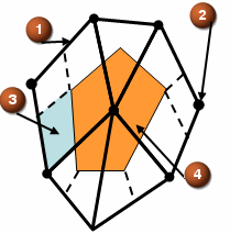
The following figure illustrates the finite volume (4) defined from elements (1) in the element-based finite volume method, [5]. All the dependent variables, including the pressure and the velocity components, are stored at the element nodes (2). This is a co-located method. Each finite volume sub-surface is an element bi-sector plane (3). In this example, a complete finite volume results from two surrounding quadrilateral elements and three triangular elements. These sub-surfaces are called integration point surfaces. The software computes the integral at their mid-points (6). This method of finite volume definition extends directly to 3D.

Diagram of a finite volume defined by three triangular elements and two quadrilateral elements, forming a heptagon.

The following figure depicts an isolated element with the integration point surfaces and the finite volume sectors.

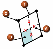
Diagram of a single quadrilateral element divided into four sections by two intersecting dashed lines.

The discretization scheme approximates the volume integrals over the element sectors and the surface integrals on the element integration point surfaces. For each element, the flow solver makes the discrete approximations to the terms in the integrals and combines them in the overall equation assembly.