How to extract and track clearances in gas turbine engines?
This article describes methods on how to extract and track clearances across the whole engine modeling (WEM).
Introduction
One of the primary purposes of a whole engine model is to calculate clearances for the entire engine, including blade tips, labyrinth seals, rim cavities, and axial gaps in the flow path. Understanding these clearances in gas turbine engines is important for predicting performance, improving efficiency, and identifying potential contact between parts. Gas turbine design teams often optimize clearances by conducting sensitivity analyses. These analyses involve varying engine geometry, materials, cooling networks, quantities, and transient engine behavior to achieve the best possible performance.
- Maximize the performance of both the turbine and compressor by maximizing the energy extracted from the flow in the turbine and the pressure ratio in the compressor.
- Maximize gas turbine efficiency.
- Understand and mitigate the risk of rubbing.
- Define rubbing allowance.
- Define cold build clearances and recommend safety margins.
- Optimize any active clearance control technology.
- Ensure aerodynamic stability in the compressor.
- Anticipate engine behavior under various operating conditions.
From WEM, you can compute radial tip, axial, and labyrinth seals clearances as shown.
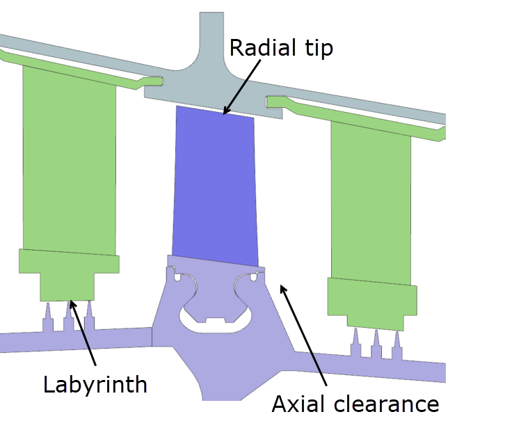
These clearances are critical for maintaining engine efficiency and preventing damage. For instance, large tip clearances allow primary flow path air to leak around the airfoil, which reduces compressor efficiency. Similarly, large seal clearances enable flow to recirculate back to the previous stage, further decreasing compressor efficiency. On the other hand, excessively tight clearances can lead to blade loss, causing vibration issues and potential destruction of downstream components. Thus, clearance analysis involves finding the optimal balance between engine efficiency and reliability.
Extracting and tracking clearance data
You can extract clearance data using one of the following methods.
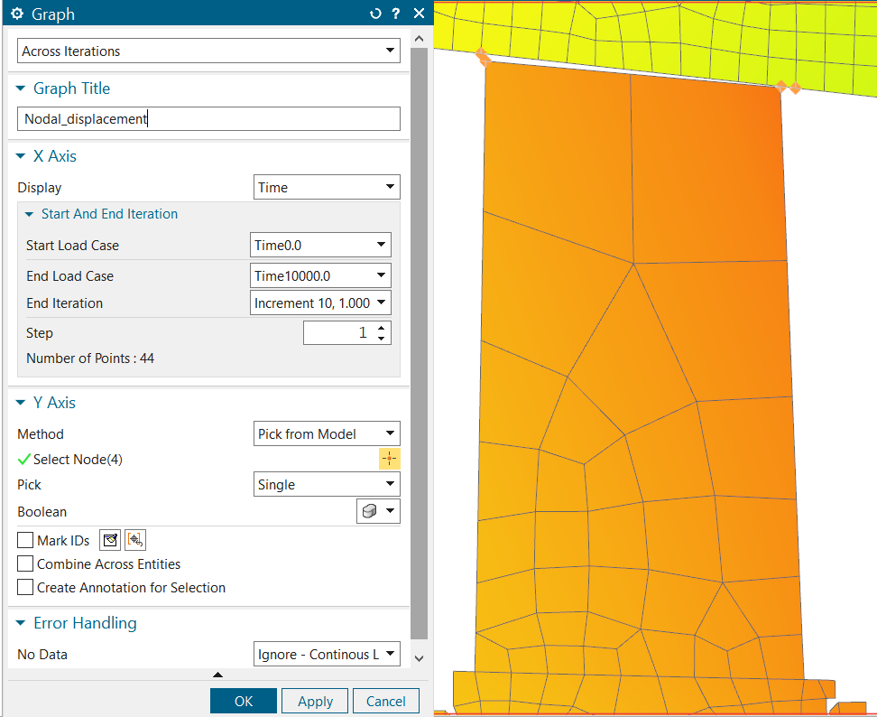
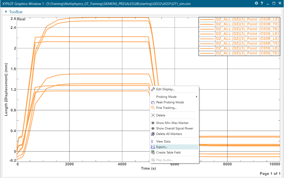
- Extracting displacements manually
- You can display the displacement results and create graphs in the
Post Processing Navigator.
- Plot the displacements.
- Choose the Create Graph command and select,
for example the leading and trailing edge nodes on the blade and
static side as shown.
- Right-click the curves in the graph and select
Export to export the data to the CSV
format.
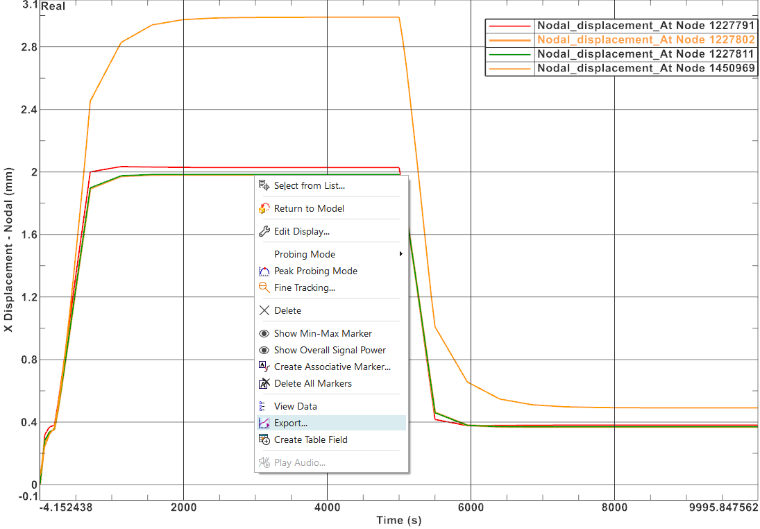
This manual method of selecting nodes during post-processing is quick and requires no advanced setup. However, it cannot be easily repeated between solves, and the data series names do not reflect the spatial location of the data. As a result, further post-processing becomes more tedious, as node numbers must be visually tracked—introducing inefficiencies and increasing the risk of errors in the analysis.
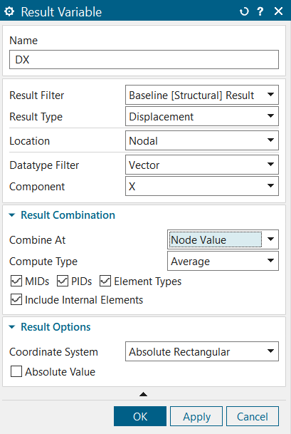
- Using result variables and result probes
- A result variable is used to reference and extract data from the solver
results file. It is then used as a definition input in a result probe
formula.
- Create a result variable, for example, for Cartesian X
displacements.
- Create a result probe, for example, on the points of the leading and
trailing edges of the compressor blade.
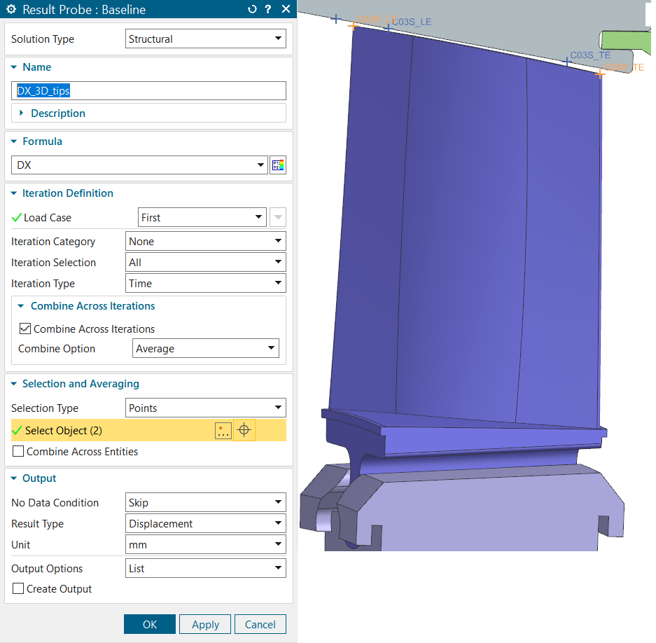
You can also create a single result probe on multiple points to extract all data at once.
- In the Simulation Navigator, right-click the result probe, and choose Create Graph to plot the graph.
- Export the graphs to the CSV format for further post processing.
- Create a result variable, for example, for Cartesian X
displacements.
- Using an expression in the result probes
- You can create an expression that calculates clearances at specific
locations and under certain conditions, for example, transient scenarios,
and reference it in the result probe.
- Use the Point command to define a point in space or on the model where you want to extract specific results before setting up result probes.
- Specify the point name by right-clicking the point and selecting Properties. For example, STATOR_1, ROTOR_1, STATOR_2, ROTOR_2, STATOR_3, ROTOR_3, STATOR_4, and ROTOR_4.
- Create a result probe and define it as a formula to extract
clearance.
- For example, to extract the cold build clearance at the
location with the minimum gap between the labyrinth seal
teeth, use the following expression:
1.2954+MINIMUM((DX("STATOR_1")-DX("ROTOR_1")),(DX(STATOR_2")-DX("ROTOR_2")),(DX("STATOR_3")-DX("ROTOR_3")),(DX("STATOR_4")-DX("ROTOR_4")))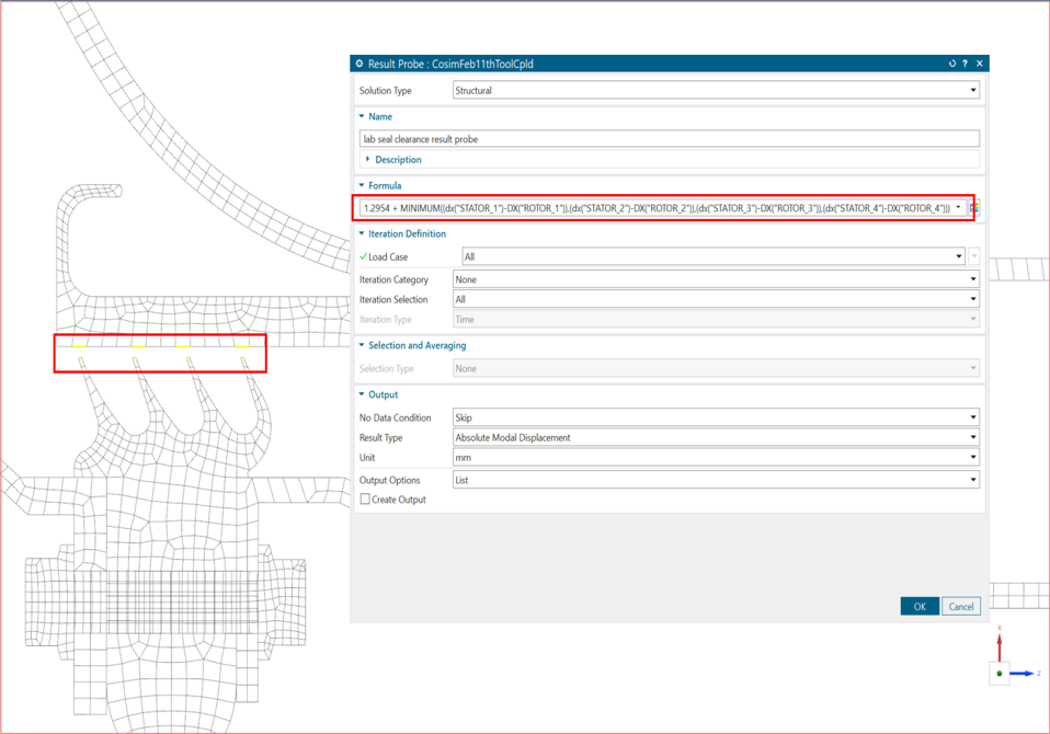
- To extract the change in the displacements in the radial and
axial directions, use the built-in functions:
DR("POINT_1")-DR("POINT_2")andDZ("POINT_1")-DZ("POINT_2")respectively.This result probe calculates the relative movement between the rotor and stator points. You can also include the cold gap based on the initial position of points, using the X() function with point names as arguments.
- For example, to extract the cold build clearance at the
location with the minimum gap between the labyrinth seal
teeth, use the following expression:
- In the Simulation Navigator, right-click the result probe, and choose Create Graph to generate a graph of the gap values at each transient time step to determine the clearance gap distance.
- Export the graph to the CSV format for further post processing.
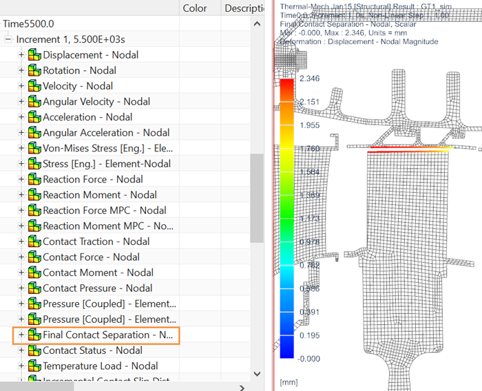
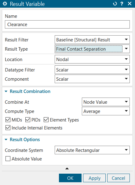
- Extracting gap distance from contact results
- The Final Contact Separation result set displays the
gap distance between the two sides of the contact boundary condition
throughout the transient cycle. To enable this request, in the
Structural Output Request, on the
Contact Result page, check Enable
BCRESULTS Request check box, and select
SEPDIS from the Separation and Slide
Distance list before solving the solution. This helps
identify potential contact points and rubbing issues.
- Create a result variable. Make sure to select Final
Contact Separation from the Result
Type list.
- Create a result probe, referencing the defined result variable.
- In the Simulation Navigator, right-click the result probe, and choose Create Graph.
- Export the graph to the CSV format for further post processing.
- Create a result variable. Make sure to select Final
Contact Separation from the Result
Type list.
Modeling clearance effects in a secondary air flow system using co-simulation
Further, you can use the extracted displacements to model clearance effects in a secondary airflow system (SAS) of the blade cooling supply network using co-simulation. You can send transient clearances from WEM to SAS and calculate off-design mass flows that may not be captured in a standard design process. For example, during a transient setup, some clearances may become extremely tight, significantly restricting mass flow and leading to elevated metal temperatures due to inappropriate cooling flow.
- Open the Co-simulation Manager dialog box to create an External Solver modeling object and all the necessary co-simulation interfaces.
- Create the External Solver modeling object to specify the path to the external SAS solver file.
- Create a Co-simulation Interface simulation object to
define a coupling interface between your 3D thermal analysis model and the
external model. You can use:
- The Custom Expression type to define a custom expression to compute a length in your model and transfer it to the external solver. You can define the custom expression using named points, expression operators, and functions.
- The Gap Distance type to transfer the gap distance between two edges or two surfaces of a 3D, 2D, or 2D axisymmetric model to the external solver. This co-simulation interface type is only available in multiphysics coupled thermal-structural solutions. You compute the gap distance using automatic or manual edge-to-edge or surface-to-surface contacts and requesting thermo-mechanical contacts.
- Activate the co-simulation solve in the Solution dialog box and launch the solve.
- (Optional) In the Solution Monitor, plot the co-simulation variables evolution. You can see the evolution of the clearance computed using the expression defined in the co-simulation interface.