To model heat load in a cavity with the assumption of uniform fluid temperature for
convection, you can use either thermal voids or duct nodes coupled to the cavity
surface.
The following table compares the two approaches.
Cavity modeling
Thermal void approach
Duct node approach
Example
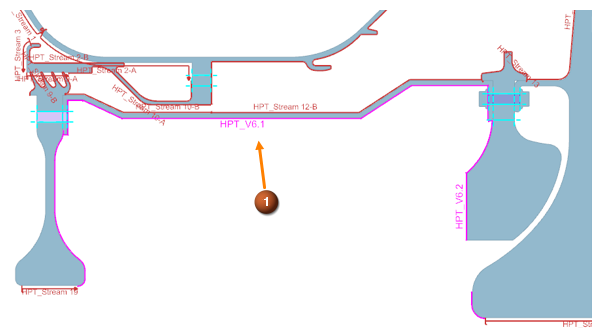
Figure 1. Using thermal void (1)
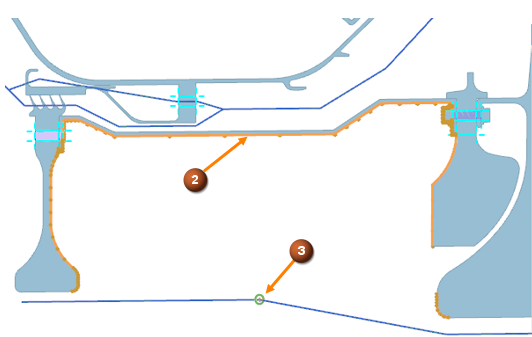
Figure 2. Using duct node(3) coupled to the surface (2)
Creation
The void represents the fluid inside the cavity. The
thermal solver generates a 0D element for the void, assuming a single
fluid temperature sink for convection.
In the FEM, you define curves and duct nodes to build a
1D duct network. Then, you mesh the ducts with 1D duct elements and the
nodes with 0D elements.
Definition
In the Simulation file, define all necessary parameters
within a single Thermal Void boundary
condition.
Convective surfaces are defined by regions.
Fluid temperature is calculated based on the region temperatures
and heat transfer coefficients (HTC).
Heat load can be used to transfer thermal energy from other
streams or sources using the PWR thermal function.
Both HTC and total temperature effect are defined in a single
dialog box.
In the Simulation file, use
The Duct Node Convection Coupling type of
Thermal Coupling - Convection to
define convective thermal coupling to connect the duct node to
the cavity surfaces.
The Duct Flow Boundary Conditions
simulation object to define mass flow, total pressure, and swirl
velocity at duct end intersections.
The Temperature constraint to define
inlet temperature on ducts.
You can:
Specify a single HTC for all surfaces within one coupling.
Define HTC with spatial variations or customize it using a
plugin.
Account for total temperature effects.
Use multiple duct nodes. If a single node is used, the behavior
is similar to a thermal void.
Advantages
Defines all required parameters within a single boundary
condition.
Reduces setup time with a unified input dialog box.
Allows for different HTCs, total temperature effects, and
pressures to be specified per region.
Allows post-processing results to be displayed at specified
locations, as the duct locations are defined in the FEM.
Enables detailed post processing analysis of interactions
between flow paths and solid boundaries.
Accepts external 1D flow solver results for direct mapping of
heat transfer coefficients.
Enables visualization of coupling connections.
Disadvantages
Requires additional work to map external 1D flow results
data.
Requires a more complex workflow, including additional steps for
FEM duct preparation.
Restricts each convection coupling to a single HTC definition
for selected convecting surfaces.
Requires additional boundary conditions for ducts at openings or
intersection locations, such as inlet temperature, total
pressures, and mass flows.