Modeling fluid network using thermal streams or ducts
This article compares thermal stream and duct modeling, highlighting the advantages
and disadvantages of each approach.
The purpose of ducts and streams are the same, to model convection between a fluid duct
and a surface, however the approaches are different as shown in the following table.
Fluid network modeling
Thermal stream approach
Duct approach
Example
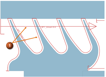
Figure 1. Modeling a labyrinth seal using thermal stream (1)
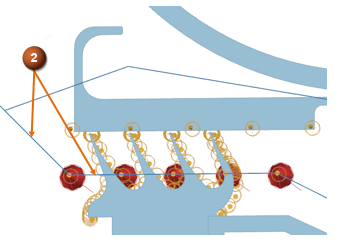
Figure 2. Modeling a labyrinth seal using ducts (2)
Creation
In the Simulation file, define all necessary parameters
within a single Thermal Stream, and then connect
the thermal streams.
In the FEM, create a 1D duct network using curves and
mesh them with 1D duct elements, which represent the flow paths.
Definition
In the Simulation file, use the Thermal
stream load to define:
Stream conditions such as mass flow, inlet temperature, and
pressure.
Heat transfer coefficient within the seal.
Heat pickup absorbed by the stream as it passes through the
seal.
Rotational effects to account for rotational loads, swirls and
compute total fluid temperatures.
In the Simulation file, you specify:
Duct Flow Boundary Conditions to define
mass flow, total pressure, and swirl velocity at duct ends
intersections.
Temperature constraint to define inlet
temperature at duct ends intersections.
Thermal Coupling - Convection to connect
the 1D duct network to surfaces and define heat transfer and
total temperature effects.
Thermal Loads to apply windage
correlation for rotating machinery effects on airflow within the
ducts.
Advantages
Automatically generates fluid elements based on wall
topology.
Defines all required parameters within a single boundary
condition.
Seamlessly integrates heat transfer, windage, and total
temperature effects.
Reduces setup time with a unified input dialog box.
Enables easy editing of stream start and end points without
modifying geometry.
Connects multiple adjacent edges by selecting just the first and
last.
Supports boundary conditions data HTML plots generation to track
thermal stream properties during solving.
Enables detailed modeling with a 1D duct network for precise
fluid flow and heat transfer control.
Provides greater control over thermal connections between duct
nodes and surfaces.
Allows specific heat transfer correlations to be applied at
different points in the network.
Eliminates the need to manually connect ducts—flow is handled
automatically.
Enables detailed post processing analysis of interactions
between flow paths and solid boundaries.
Accepts external 1D flow solver results for direct mapping of
heat transfer coefficients.
Allows a more streamlined workflow for mapping data from 1D
results.
Supports various driving forces: velocity, flow rate, mass flow,
or pressure rise.
Automatically calculates head loss from curvature, bends, and
junctions.
Allows thermal convective coupling at nodes.
Models convection with ducts immersed in the solid body using
Immersed Ducts.
Disadvantages
Requires manual setup of multiple streams and junctions to build
the fluid network.
Limited to defining mass flow as the driving condition.
Lacks the capability to visualize the fluid network before
solving during pre-processing.
Requires additional boundary conditions for ducts at openings or
at intersection locations such as inlet temperature, total
pressures, and mass flows.
Involves a more complex workflow with additional steps for FEM
duct preparation.
1D fluid temperature
results
The solver automatically creates 1D fluid ducts during
the solve, with no user control over their location. Post-processing
results are shown on these solver-created ducts.
Duct locations are predefined in the FEM.
Post-processing results are displayed at these specified
locations.