Calculation of ray intercept and direction for curved elements

This topic describes the procedure for calculating the local surface normal, the point of interception, and the new ray direction for curved elements.

Curved elements are parabolic elements, defined by specifying the midside nodes of the sides.

The shape of the surface is represented using the standard finite element parabolic shape functions. These describe the variations of x, y, and z on the surface as functions of 2 parameters: s and t. The equation for the shape of the surface is defined by curve-fitting the coordinates of the nodes.

1. The thermal solver identifies the sub-triangle within the element which the ray intersects.

   

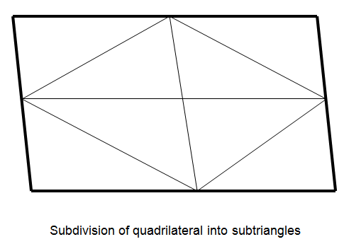
2. For quadrilaterals, the thermal solver selects a point at the parametric center of the element (s=0, t=0) and determine its x, y, z coordinates. Using this point and the 8 element nodes, it subdivides the quadrilateral into four quadrants. Subdivide each quadrant into two, yielding 8 sub-triangles, and determine which sub-triangle the ray intersects.

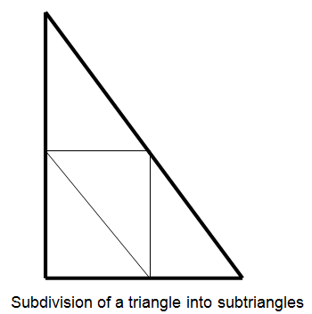
   If the element is a triangle, it is not subdivided, but is considered to be the intersecting sub-triangle.

3. The thermal solver subdivides the intersecting sub-triangle into 4 more sub-triangles by connecting the midpoints of the sides. It determines which sub-triangle the ray passes through and calculates the surface normal of the sub-triangle and the intersection point with the ray, assuming the sub-triangles are planar.

   

4. The thermal solver calculates the new intersection point and surface normal for this sub-triangle, assuming the sub-triangle is planar.
5. It defines a tolerance parameter D:
6. The thermal solver compares results from the subdivision of Step 2 and Step 3.

   If the intersection point has moved less than D and the angular change in surface normal is less than 0.01 radians, then stop. Otherwise, subdivide again and start with Step 2.

7. It handles cases where the ray does not intersect an element or a sub-triangle.

   If during the intersection calculations the ray does not intersect an element or a sub-triangle, then the element or sub-triangle is expanded in parametric space and the intersection calculation is restarted. The expansion is applied recursively until an intersection is found or an internal limit is reached.

8. The thermal solver calculates the reflected ray using the point of interception and the local surface normal once the point of intersection has been determined.

   The new ray is then checked to see if it re-intersects the same element. The reflection/re-intersection procedures are repeated until a new ray does not re-intersect the element or 5 bounces are found.

9. The thermal solver handles failure in the curved element processing.

   In the event of failure in the curved element processing, the thermal solver resorts to using the planar approximation to the element.

10. Once the direction and strengths of the ray launched from j are established, an artificial 1-node element k' is created at a very large distance along the ray. All the shadowing surfaces are then checked for interception of the ray originating at DA_j and ending at k'. If more than one shadowing surface intercepts, the one with the point of interception closest to DA_j is chosen as the intercepting surface.

    Next, a search is done within the intercepting shadowing surface to identify the element k that is hit, and the coordinates of the interception point are computed.

    If the ray is not terminated, new strength values and directions are calculated in the manner described above, and the ray is further continued.