View factors calculation using the hemicube method

The thermal solver uses the hemicube method to compute diffuse blackbody view factors.

Cohen and Greenberg [32] first proposed the hemicube algorithm, in which the five sides of an imaginary hemicube cover an element such that the center of the cube is at the centroid of the emitter element i, and the top plane of the cube is parallel to the plane of the element. The following example shows projection of two elements onto hemicube.

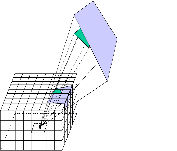
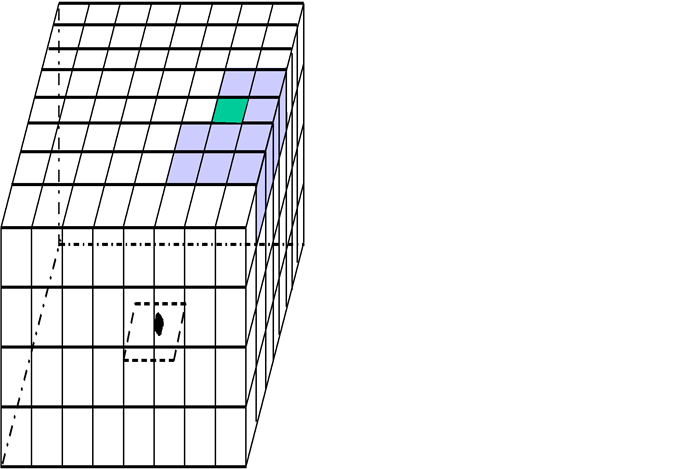
The faces of the hemicube are divided into equal size squares, referred to as pixels, with areas of dA. Each element j, called the receiver element, is graphically projected onto the faces of the hemicube, with the focus of the projection on the centroid of emitter element i. This projection is easily and efficiently performed within computer graphics hardware, with each hemicube face containing the rendered image of a section of the model.

Each receiver element j is assigned a unique color, and a depth-buffer algorithm (Z-buffer) ensures that only the visible parts of overlapping elements appear in the final image. The rendered images on the five hemicube surfaces comprise the images of all the elements of the model surrounding the emitter element i. The pixel colors of these five images are post-processed to calculate the view factors of the emitter i to each element.

This example depicts two elements being rendered onto the surface of a hemicube, and the resulting pixel colors after the rendering process.

Calculation of view factors

Each pixel is associated with a pre-computed delta view factor ΔF_p,

where the geometry is shown on the following figure.

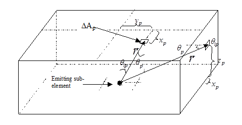
The vector r is from the eye position (CG of the emitting element i) to the CG of the pixel under consideration. θ_ip is the angle between r and the emitter element normal. θ_p is the angle between r and the normal to the hemicube plane on which the pixel lies.

A pixel’s contribution to the view factor, is derived by assigning a local (x,y,z) coordinate system to the hemicube, and making the hemicube a unit height. Then, for pixels on the top plane of the hemicube,

Substituting these equations to the equation for ΔF_p:

for top plane pixels of uniform area ΔA. Similarly, for the side plane pixels:

which yields:

The rendering procedure

First, the eye position, view direction, viewing frustum dimensions, and image plane location parameters are defined. The eye position is at the CG of the emitter element i. The view direction is perpendicular to each of the viewing planes, i.e. the sides of the hemicube. The top surface of the viewing frustum is a side of the hemicube, the bottom surface is a corresponding square or half-square located at the emitter CG.

Next, the colors and vertex coordinates of the j elements are processed for rendering. Each receiver element, as well as its reverse side, is assigned a different color. Finally, a “draw” command is issued, and the graphic hardware draws the receiver element images on the five rendering planes, as seen from the position and perspective of the CG of the emitter element i.

The thermal solver uses the following workflow for image rendering.

Once these initial parameters are set, the algorithm loops over all the sides and all the receiver elements j, projecting them onto the five sides.

If a reverse side is not defined, it is still projected onto the rendering planes, but the view factor to it are discarded and a warning message is issued.

For greater accuracy and efficiency, only view factors from smaller to larger elements are considered.

After the image is rendered, the view factors are computed by summing the pixels of different colors in each of the five views. The contribution of a pixel to the view factor f_ij between elements iand jof the hemicube view l is computed with:

where ΔF^l_lk is the delta view factor for pixel k of hemicube view l and H_jk is the Heaviside function which equals 1 when the color of pixel k matches the color of element j, and 0 otherwise.

Using the MESH parameter

The accuracy of a view factor calculated with the hemicube method decreases if two elements are close together, i.e. if the view factor between them is large.

If one does not use a MESH ERROR setting, then for each element i the following iterative procedure is employed. First, all the view factors are calculated with no elemental subdivision, i.e. the emitter element is not subdivided. Next, an evaluation is performed. If a view factor seen through the top viewing plane is > .03, or the view factor seen through the side viewing plane is > 0.3, a second run is performed, with the MESH parameter specified by the user. If desired, one can bypass this check of view factor values and enforce unconditional use of the specified MESH parameter by activating an Advanced Solver Parameter (EMS) or specifying the Card 9 GPARAM 56 38 1.

If a MESH ERROR value is defined, then, regardless of the above MESH parameter setting, the mesh size for the elemental subdivision is determined automatically for each element so that the view factor sum error would be approximately within the given MESH ERROR set tolerance. This is the recommended option since it allows maintaining consistent accuracy throughout a model with different element sizes and configurations in it, while also minimizing the computational cost to achieve a given overall accuracy level. The MESH ERROR algorithm uses a view factor sum error estimate that is based on view factor values calculated without elemental subdivisions, distances from a given element to its surrounding elements, and the area of the given element. That error estimate uses a view-factor weighted direction average of estimated view factor errors for all emitter-receiver element pairs for a given emitter element.

The final view factor is calculated by summing the view factors of all the sub-elements:

where

dA_l is the m^th incremental area of emitter element i.
f^m_i-j is the view factor for the m^th incremental area of element ito element j.

Choosing the winsize parameter

The rendering window size is specified by the WINSIZE parameter. WINSIZE defines the number of pixels that can be drawn on the screen, and hence affects the accuracy of the view factor calculations, the maximum number of elements that can be drawn, and total CPU time the module may take.

The total number of pixels for the top view is WINSIZE*WINSIZE, for the side view is WINSIZE²/2. The maximum number of colors (and hence the maximum number of elements that can be drawn, i.e. seen by a given element) is 5*WINSIZE². Please note that more elements than this can exist in a model, provided that some of these elements shadow each other.

A larger WINSIZE value will increase the accuracy of the calculation but will also increase the CPU time. The default WINSIZE value is 128, which corresponds to a maximum of 49,152 elements that can be seen by any given element through one of the viewing planes.