Radiative conductance calculation methods
Radiative conductance defines the rate (W/K) at which thermal radiation is exchanged between surfaces. The thermal solver supports multiple methods for calculating radiative conductance, each suited to different levels of geometric complexity, material properties, and computational constraints.
Because view factors only account for geometric relationships between surfaces, they are insufficient on their own to determine radiative heat transfer. Accurate surface‑to‑surface radiation modeling must also consider emission, absorption, and reflection effects.
The solver models radiative exchange as an electrical network, where surfaces are treated as nodes and radiative conductances connect them. It identifies surface pairs that exchange radiation and solves the resulting system to determine heat flow.
This approach linearizes the Stefan-Boltzmann law, σT4, around a reference temperature, Tref, to create a temperature-dependent radiative conductance network.
where Gij(Tref) is a function of the reference temperature Tref, representing the linearization of the nonlinear term (Ti4-Tj4).
At each iteration, the solver recomputes the temperature‑dependent radiative conductances Gij from the current surface temperatures. Each Gij depends on temperatures at the current iteration and the geometry via view factors. These conductances are assembled into the global matrix exactly like conduction terms.
Finite volume and finite element conductance calculation approaches
In the finite volume method (FVM), the solver determines the radiative conductances from fluxes exchanged across control volumes. Each face represents a discrete area through which radiation is emitted, absorbed, or reflected. The radiative conductance network is constructed by relating these face-based fluxes, ensuring local energy balance at the control-volume level.
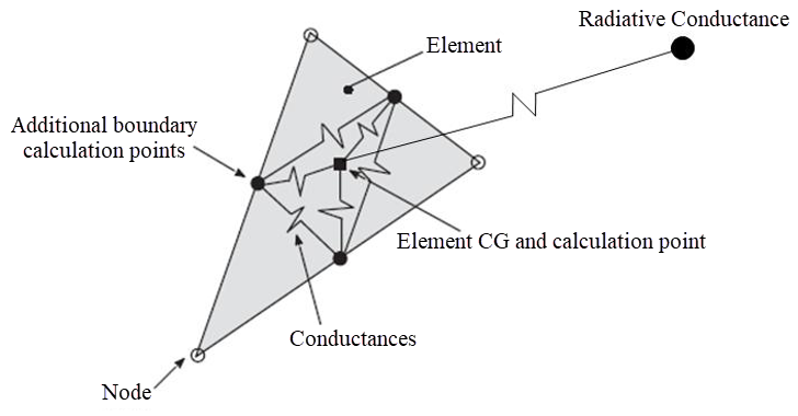
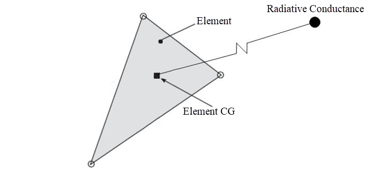
In the finite element method (FEM), the solver evaluates the radiative exchange using element level temperatures instead of nodal integration of boundary fluxes. This modification simplifies the system by reducing matrix connectivity and improving computational efficiency, while maintaining sufficient accuracy within the FEM framework.
Each element exchanges radiation through a radiative conductance associated with its temperature field. The temperature applied in the calculation is evaluated at the element’s centroid (CG) by interpolating nodal values using FEM shape functions.
For both FVM and FEM, the thermal solver computes radiative conductances using one of the following methods: Gebhart’s, Oppenheim, or Monte Carlo. Both FVM and FEM rely on the same physical models for surface‑to‑surface radiation; they differ only in how conductances are incorporated into numerical system.
Methods for computing radiative conductances
- Gebhart’s method
-
Gebhart’s method builds upon view factors by solving a system of equations that accounts for multiple reflections and interactions between surfaces.
- Computational cost: Requires solving N systems of N equations, which can be computationally expensive.
- Matrix characteristics: Produces a dense matrix with many small terms, leading to high memory and storage demands.
- Advantage: Provides a clear and intuitive understanding of heat flow paths.
- Limitation: Not suitable for materials with temperature-dependent material properties.
- Oppenheim radiosity method
- The radiosity method introduces additional unknown variables to model
surface radiosity, which includes both emitted and reflected radiation.
- Computational cost: Adds N more unknown variables to the system, increasing the size but not necessarily the complexity.
- Matrix characteristics: Results in a relatively sparse matrix, which is more efficient to store and solve compared to Gebhart's method.
- Advantage: Supports temperature-dependent emissivity, making it suitable for more realistic material modeling.
- Limitation: The resulting heat flow paths are less intuitive compared to Gebhart’s method.
- Monte Carlo method
-
The Monte Carlo method uses statistical sampling to simulate the paths of many radiation particles, making it highly flexible and accurate for complex geometries and optical properties.
- Computational cost: Computationally intensive due to the large number of samples required for accuracy.
- Matrix characteristics: Produces a matrix similar in size and form to that of Gebhart’s method.
- Advantage: Well-suited for systems with direction-dependent or spectrally varying optical properties.
- Limitation: Not ideal for temperature-dependent material properties due to the complexity of integrating such dependencies.
Comparison
The following table summarizes the key characteristics of the radiative conductance methods.
| Criterion | Gebhart’s method | Monte Carlo method | Oppenheim radiosity method |
|---|---|---|---|
| Computational cost | High | High | Moderate |
| Matrix characteristics | Dense, many small terms | Dense, similar to Gebhart’s | Sparse |
| Supports temperature-dependent properties | No | No | Yes |
| Suitable for complex optical properties | No | Yes | Yes |
| Ease of interpreting heat flows | Easy | Moderate | Hard |