Oppenheim method

The thermal solver can compute radiative conductances using the Oppenheim method.

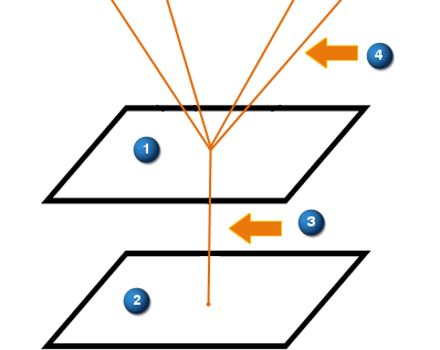
The Oppenheim method, or otherwise known as the radiosity method, is the recommended approach. The Oppenheim method consists of creating an artificial Oppenheim element I (1) for each radiating element k (2), which may be visualized as an imaginary element floating above element k, and intercepting all radiation to it (4).

A radiative coupling (3) is created between I and k, and each view factor VF_kj is transformed into a radiative coupling (4) A_kVF_kj between I and the Oppenheim element J of element j.

The Oppenheim method is an alternative to the Gebhardt method for calculating radiative couplings. It has several advantages:

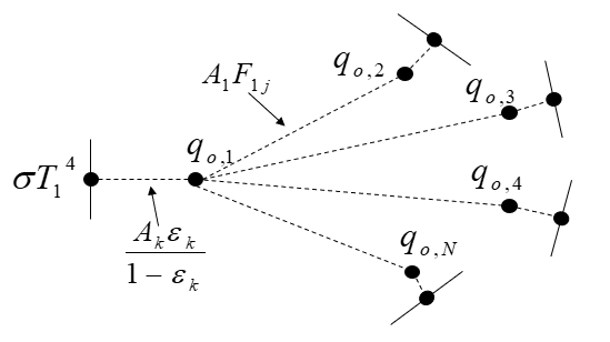
• Temperature-dependent emissivities are handled more accurately and efficiently. This is because during temperature calculations only the radiative conductance A_kϵ_k/(1−ϵ_k) between the Oppenheim element and the element itself needs to be modified.
• CPU performance is generally better because the matrix inversion process of the Gebhardt method is bypassed, and the number of radiative couplings is generally much smaller. This is because, in an enclosure, the Gebhardt method creates a radiative coupling between every element, even when no direct view exists between them.
• Accuracy is improved because the elimination of insignificant radiative couplings, which is used in the Gebhardt method, is bypassed.
• File sizes are generally smaller.

With the Oppenheim method, significant performance degradation can be expected during transient analysis with the explicit forward differencing method. This is because the Oppenheim elements are assigned zero capacitance, and the forward differencing method requires a full steady-state solution for the surface elements at each integration time step.

However, no accuracy degradation is observed with the implicit time integration methods.

This method defines the radiosity as the total energy flux leaving a surface, which includes both emitted and reflected radiation:

where:

• q_o,k is the outgoing radiosity flux from surface element k.
• ε_k is the emissivity of surface k.
• σ is the Stefan-Boltzmann constant.
• T is the absolute temperature of the surface.
• ρ_k is the reflectivity of surface k.
• q_i,k is the incoming radiative flux to surface k.

The incoming flux is computed as a sum of contributions from all other surfaces using view factors:

Where F_kj is the view factor from surface k to surface j.

The net heat transfer to surface element k is then given by the difference between outgoing and incoming fluxes, multiplied by the surface area:

The radiosity equation can be expressed in a form that relates the outgoing flux from a surface element to the difference in radiosity between that element and all others in the system. The net radiative heat exchange for surface k:

Oppenheim elements are created to carry the unknown radiosities. The thermal solver uses “temperature,” rather than radiosity as the unknown variable for the Oppenheim element.

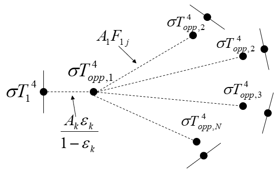
The radiosity equations are linearized and integrated into the thermal conductance matrix. This allows the radiative exchange to be solved simultaneously with the temperature field.

To ensure energy balance across all surfaces, the following equation is used:

These equations are assembled into a global matrix system of the form where first matrix is the conductance matrix [G]: