Wall boundaries

The flow solver treats both slip or no-slip wall boundaries identically in the particle transport problem. However it applies different boundary treatments depending on the particle impact type.

Figure below depicts the case when the particle, shown in red, reaches a wall boundary δΩ_i. In the flow solver, the impact, denoted by , is approximated as an instantaneous event at time t_bnd.

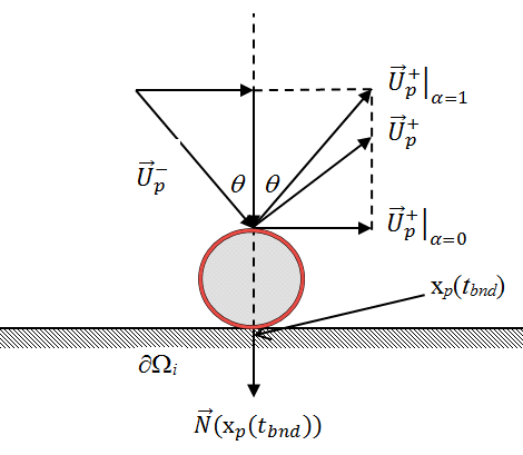
Denote the particle approach velocity predicted by the integration of the particle motion equations and the departure velocity after application of the boundary treatment, respectively as:

The flow solver applies different boundary treatments depending on the particle impact type:

1. At walls with particle impact type set to stick, when the particle reaches the wall boundary, the wall-normal component of particle velocity regardless of and the particle continues to be counted towards the statistics, so that an accumulation of particle density at the wall is captured.
2. At walls with particle impact type set to rebound, when the particle reaches the wall boundary, the wall-normal component of particle velocity is modified as follows, using the collision model with the coefficient of restitution α ∈ [0, 1] [32]:

where is the outward unit normal vector to the boundary surface for all x ∈ δΩ_i.

The coefficient of restitution is a measure of the portion of the energy associated with the wall normal component of the approach velocity, which is retained after the collision. For a purely elastic collision, α = 1 and the particle is reflected off of the wall with no loss of energy. When α = 0, the particle loses all wall-normal momentum during the collision.

The integration of the particle motion equations is then continued from the predicted location , with the imposed velocity .

The flow solver continues to track particles that stop at walls and considers these particles in the output statistics.