Guidelines for modeling lenses in thermal simulations
This article outlines strategies for modeling lenses in thermal simulations, particularly when considering optical performance, thermal effects, and radiative properties.
- 2D shell modeling
- 3D solid modeling
- 3D solid modeling with 2D coating
- 3D solid modeling with 2D coating and with defined extinction coefficient
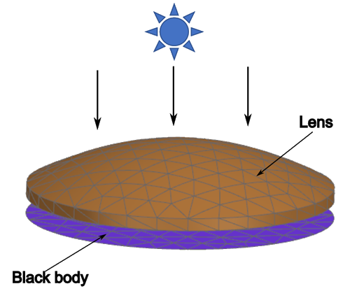
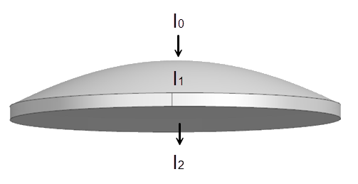
- A lens with a total absorptivity of 0.05 and transmissivity of 0.95.
- Solar Heating Space applied directly overhead at 100 W/m2.
- A receptor, modeled as a black body, placed beneath the lens to capture the
transmitted solar flux.
2D shell modeling
Use this simplest method when you need a quick, first-order approximation of lens behavior, and when focusing effects and internal thermal gradients are not relevant in the analysis.
- Modeling approach
-
- Represent the lens as a 2D shell with no curvature or thickness.
- Define transmissivity equal to the real total lens transmissivity and absorptivity for both front and back sides.
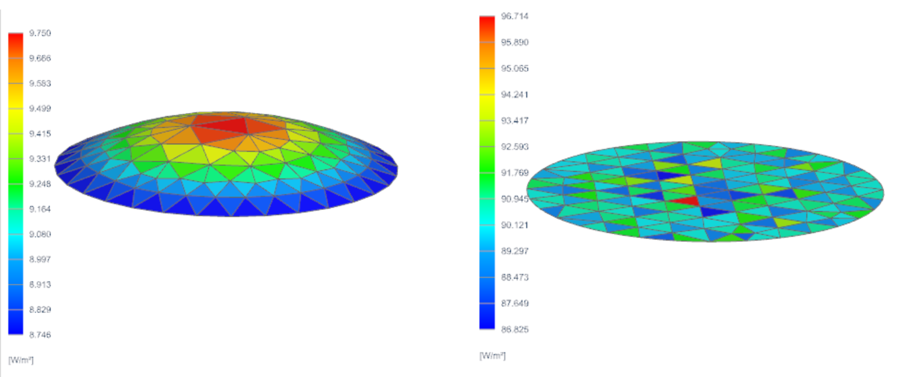
- Results
-
The lens absorbs approximately 9 W/m2 of the incoming flux on average, while the black body beneath it captures an average of 90 W/m2 of transmitted solar flux.
3D solid modeling
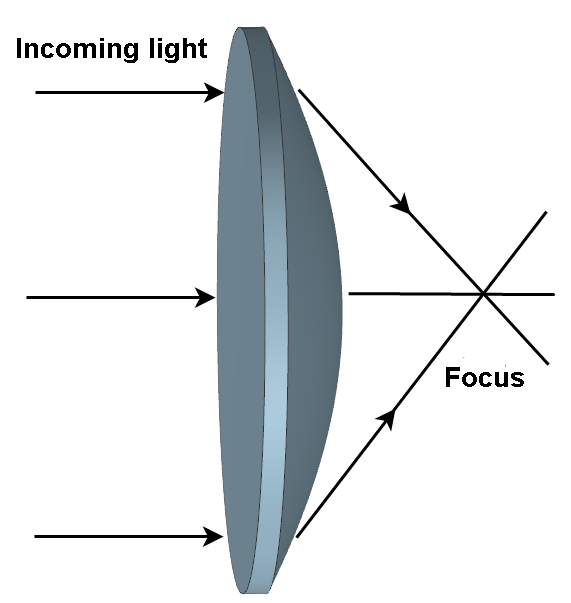
You can model focusing effects using a 3D solid lens.
- Extinction data is unavailable and you want a first-order approximation of how front-surface heating redistributes by conduction.
- The lens is very transparent and you expect nearly all absorption to occur at the first interface.
- Conduction through geometry is the main interest, not where inside the lens the absorption takes place.
- Modeling approach
-
- Mesh the lens with 3D solid elements to represent shape and thickness.
- Enable radiation in the 3D mesh collector, and define
transmissivity and absorptivity equal to the real total lens
transmissivity and absorptivity.
Note that radiative properties such as transmissivity (T), absorptivity (A), and reflectivity (R) are not applied directly to the solid elements. This is because solid elements do not participate in radiation calculations. Instead, the thermal solver automatically generates 2D coating elements on the exposed surfaces of the solids. These coatings are used by default for all radiative heat transfer and view factor calculations, if the solid surfaces are selected. In this setup, the thermal solver applies radiative properties only to one side of the solid, and treats the opposite side as fully transparent.
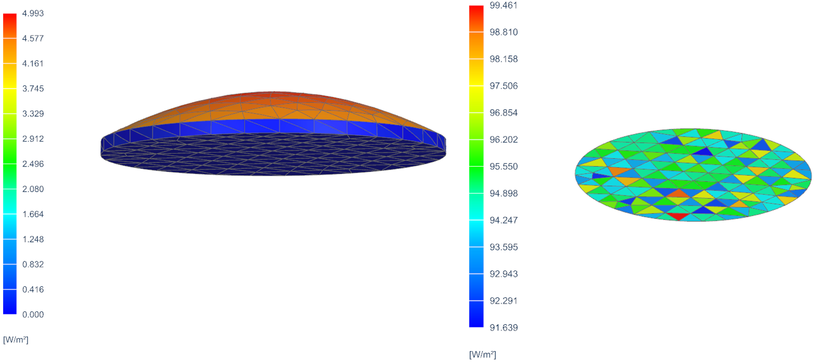
- Results
-
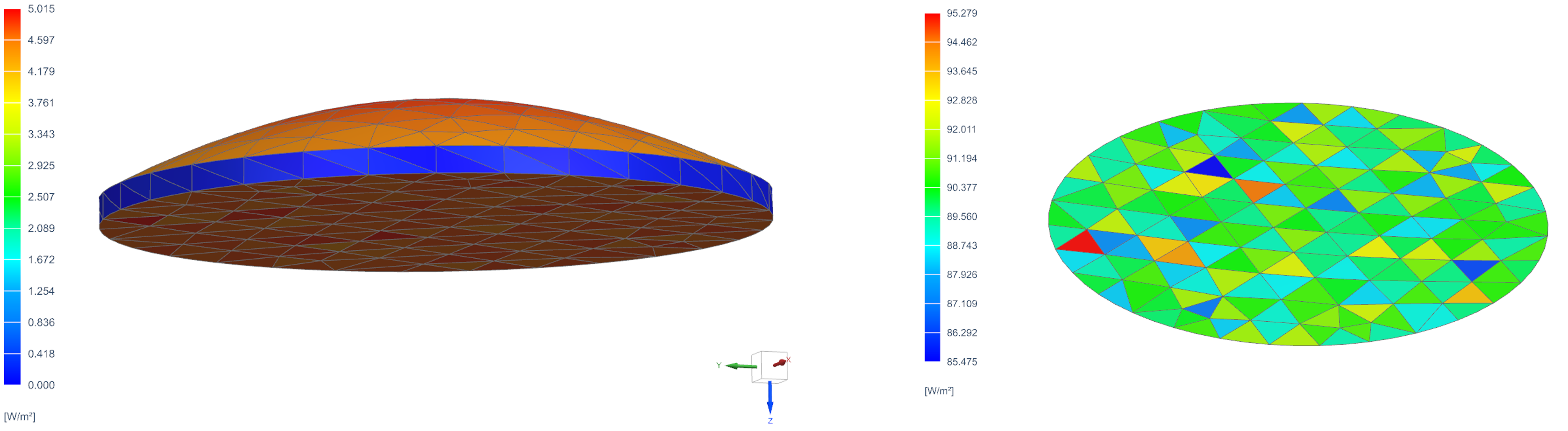
The top of the lens captures 5% of the flux, the rest makes it onto the black body (avg 95W/m2). The reverse side of solid element faces is considered fully transparent by the solver, even if they’re selected in the bottom region of the solar heating object.
Use shell coatings on each side of the lens to capture ray bending and curvature while controlling optical properties without modeling internal conduction or absorption. By default, the solid elements are treated as transparent to radiation, and ray tracing is performed between the coating layers. The solids contribute only to thermal conduction through the lens thickness.
- Modeling approach
-
- Mesh the lens with 3D solid elements to represent shape and thickness.
- Apply 2D shell coatings to the front and back faces.
- Radiation passes through the solid; absorption occurs in the coatings, with heat transferred to the solid by conduction.
- Define front and back side refractive indices; these are the refractive indexes of the material on the respective side of those shells.
- Define the per-surface optical properties, such as
transmissivity, absorptivity, and reflectivity, so that the
combined effect of the two 2D surface elements (front and back
of the lens) reproduces the total optical behavior of the real
3D object. The method used to calculate these values is
described in the Computing optical properties section.
The transmissivity for each thin shell mesh coating should be the square root of the total lens transmissivity.
- Results
- Both the top and bottom surfaces of the lens absorb ~5% of the flux,
with ~90 W/m² reaching the black body.
Including or excluding the reverse sides of coating elements in the solar heating setup has no impact on the results; the ray-tracing method accounts for this automatically.
Computing optical properties
To approximate a real 3D lens using two 2D surface elements, you must assign transmissivity (T), absorptivity (A), and reflectivity (R) to each surface so that, when combined, they reproduce the overall optical response of the physical lens. At each surface, these properties must satisfy the energy balance.
- is transmissivity, fraction of light transmitted through the material.
- is absorptivity, fraction of light absorbed by the material.
- is reflectivity, fraction of light reflected by the surface.
- Without Reflection (R=0)
-
This simplified model assumes no light is reflected, only absorbed or transmitted.
Assume that:- is the total transmissivity through a full lens.
- is the total absorptivity through the full lens.
- is the incident light intensity.
- is the transmissivity per surface.
- is the absorptivity per surface.
- With reflection (R>0)
- When surface reflectivity is significant, reflected energy must be
incorporated into the energy balance. It is necessary to explicitly account
for all three optical properties at each surface: Where:
- is the transmissivity per surface.
- is the absorptivity per surface.
- is the reflection per surface.
The cumulative total properties are computed based on the overall energy balance across both surfaces.
The first surface reflects , absorbs , and transmits , which then becomes the incident light intensity for the second surface.
The second surface reflects , absorbs , and transmits .
The total transmission is the same as in the non-reflective case, since reflection does not affect the portion of light that is already transmitted. Thus, .
The total absorption is:
The total reflection is:
| Property | Formula | Comments |
|---|---|---|
| Assumes front and back surfaces are identical. | ||
| with reflection | Distributes absorption across two passes. Used when reflection is included. | |
| without reflection | Derives from conservation of energy . Used when reflection is zero. | |
| Applies as a linear approximation for small absorption <<1. | ||
| Assumes no multiple internal reflections. |