VVC6 - Forced convection in a rectangular duct
| Case A: Temperature constraint | Case B: Heat flux load | |||
|---|---|---|---|---|
| α* | Mesh | Test case | Mesh | Test case |
| 0.1 | Coarse | SVTEST60 | Coarse | SVTEST61 |
| Fine | SVTEST62 | Fine | SVTEST63 | |
| 0.2 | Coarse | SVTEST64 | Coarse | SVTEST65 |
| Fine | SVTEST66 | Fine | SVTEST67 | |
| 0.3 | Coarse | SVTEST68 | Coarse | SVTEST69 |
| Fine | SVTEST70 | Fine | SVTEST71 | |
| 0.4 | Coarse | SVTEST72 | Coarse | SVTEST73 |
| Fine | SVTEST74 | Fine | SVTEST75 | |
| 0.5 | Coarse | SVTEST76 | Coarse | SVTEST77 |
| Fine | SVTEST78 | Fine | SVTEST79 | |
| 0.6 | Coarse | SVTEST80 | Coarse | SVTEST81 |
| Fine | SVTEST82 | Fine | SVTEST83 | |
| 0.7 | Coarse | SVTEST84 | Coarse | SVTEST85 |
| Fine | SVTEST86 | Fine | SVTEST87 | |
| 0.8 | Coarse | SVTEST88 | Coarse | SVTEST89 |
| Fine | SVTEST90 | Fine | SVTEST91 | |
| 0.9 | Coarse | SVTEST92 | Coarse | SVTEST93 |
| Fine | SVTEST94 | Fine | SVTEST95 | |
| 1.0 | Coarse | SVTEST96 | Coarse | SVTEST97 |
| Fine | SVTEST98 | Fine | SVTEST99 | |
Description
This verification case examines forced convection heat transfer inside a rectangular duct. The flow is operating in a laminar flow regime. It is assumed that the flow is fully developed over most of the duct length, which allows for a significantly simplified analysis of the heat transfer parameters. Two different thermal boundary conditions are considered:
- Case A: Constant temperature duct walls
- Case B: Constant heat flux duct walls
The results predicted by the solver are compared with the analytical solution.
Geometry
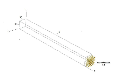
The model geometry includes the duct widths (W), ranging from 0.1 m to 1.0 m, the fixed duct length (L) = 15.0 m, and the fixed height (H) = 0.1 m. The following figure presents the geometry in detail.

Simulation model
The model is meshed with solid hexahedral elements and 4-node planar elements. Two different mesh densities are used for both sets of thermal boundary conditions and presented in the following table.
| Mesh type | Elements per L=15 m | Elements per W=0.1m to 1m | Elements per H=0.1m | Fluid element size |
|---|---|---|---|---|
| Coarse | 50 | 1 per 0.02m of W | 5 | 0.3x0.02x0.02 |
| Fine | 100 | 1 per 0.01m of W | 10 | 0.15x0.01x0.01 |
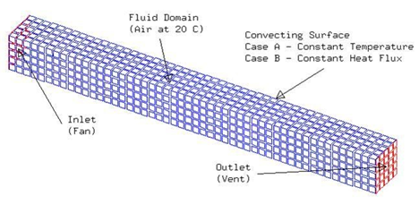
4-node 2-D elements are used to define the mesh density of the duct inlet side at Z = 0 m. A 3D mapped mesh technique, using 8-node hexahedral elements, is then used to create the fluid mesh between the inlet and outlet (opening) of the duct. Once completed, the 4-node 2-D elements are deleted since they are not used by the solver, as null shells are automatically created for the duct walls. The mesh is presented in the following figure.

The fluid is modeled using air with the following properties:
- Mass density: ρ = 1.207 kg/m3
- Thermal conductivity: k = 0.0263 W/m·K
- Dynamic viscosity: µ = 1.85e-005 kg/m·s
- Specific heat at constant pressure: Cp = 1007 J/kg·K
- Coefficient of thermal expansion: β = 3.41e-3 K-1
- Gas constant: R = 287 J/kg·K
The following boundary conditions are applied:
- Flow Boundary Condition: Inlet Flow on the Z face polygon at a distance Z = 0m with velocity V m/s. The velocity V for the various duct widths is calculated based on a Reynolds number of 652
- Flow Boundary Condition: Opening on to the outlet at a distance Z = 15m
- Flow Surface: Boundary Flow Surface on the four duct surfaces using the No Slip Wall option with smooth wall friction and convection properties set to Automatic
- Temperature constraint (Case A) on the four polygon surfaces defining the two sides, top and bottom of the duct with a value of T = 100 °C
- Thermal Load: Heat Flux (Case B) on the four polygon surfaces defining the two sides, top and bottom of the duct with a value of q = 10 W/m2
The following non-default solver options are used:
- Turbulence Model: None( Laminar Flow)
- Buoyancy: Not activated
- Solution Type: Steady State
- Ambient Conditions: Fluid temperature = 20 °C, absolute pressure value = 0.101351 MPa
The following non-default solver parameters are used:
- 3D Flow Solver: Physical steady-state with time step = 2 s
- 3D Flow Solver: Maximum Residuals = 1e-4
- Coupled Solver: Max temperature change = 0.1 Δ°C
- Coupled Solver: Global heat imbalance fraction = 0.01
Theory
The velocities, V, for the various duct widths are calculated based on a Reynolds number of 652.
where:
- H is the duct height.
- W is the duct width.
According to the theory, the Nusselt number of forced laminar fully developed flow in an isothermal rectangular duct or in a rectangular duct with a constant heat flux at the wall, is constant and is a function of the aspect ratio of the duct cross-section, α*, only [39].
The Nusselt number for constant wall temperature (Case A), NuT, is defined as:
The mean heat flux coefficient, hm, is defined as:
where:
- q is the total amount of heat transferred to the fluids.
- At is the total contact area.
and ΔTlm is the average of the temperature difference over the duct length, determined from [40] as:
where Tw is the duct wall temperature, and Tmi and Tmo are the mean inlet and outlet temperature of the fluid, respectively.
For fully developed flow, the Nusselt number in a rectangular duct with uniform wall temperature, can be approximated by the following empirical equation [39]:
The theory of Shah and London [51] is used as a basis of comparison for constant heat flux at duct walls boundary conditions (Case B) solver results.
Results
In order to calculate the Nusselt number from the solver results, the fluid mean outlet temperature Tmo and the amount of heat convected to the fluid q are required. The total heat convected to fluid can be found in the solution summary section of the text log file. The fluid mean outlet temperature, Tmo and mean inlet temperature Tmi are evaluated from the following equations:
where:
- nnode is the number of nodes across the plane.
- Vi is the velocity magnitude at node i.
- Ti is the fluid temperature at node i.
The following table summarizes the data used for the case A: constant temperature on duct walls solution.
| α* | W (m) | Dh (m) | Vin (m/s) | qcoarse (W) | qfine (W) | Tmo,coarse (°C) | Tmo,fine (°C) |
|---|---|---|---|---|---|---|---|
| 0.1 | 1.0000 | 0.18182 | 0.055 | 505 | 510 | 98.55 | 98.85 |
| 0.2 | 0.5000 | 0.16667 | 0.060 | 273 | 277 | 97.07 | 98.39 |
| 0.3 | 0.3333 | 0.15385 | 0.065 | 196 | 198.5 | 97.69 | 98 |
| 0.4 | 0.2500 | 0.14286 | 0.070 | 158 | 160 | 97.48 | 97.75 |
| 0.5 | 0.2000 | 0.13333 | 0.075 | 135 | 136.7 | 97.46 | 97.68 |
| 0.6 | 0.1667 | 0.12500 | 0.080 | 121 | 121.5 | 97.58 | 97.75 |
| 0.7 | 0.1429 | 0.11765 | 0.085 | 110 | 110.9 | 97.77 | 97.93 |
| 0.8 | 0.1250 | 0.11111 | 0.090 | 102 | 102.9 | 97.91 | 98.17 |
| 0.9 | 0.1111 | 0.10526 | 0.095 | 95.9 | 96.7 | 98.21 | 98.43 |
| 1.0 | 0.1000 | 0.10000 | 0.100 | 91.2 | 92 | 98.53 | 98.68 |
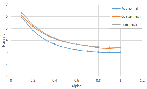
The following table and figure present the comparison of average Nusselt numbers predicted by the solver with the theoretical data for constant temperature duct walls.
| α* | Nucorr | Nucoarse | Errorcoarse (%) | Nufine | Errorfine (%) |
|---|---|---|---|---|---|
| 0.1 | 5.9110 | 6.0719 | 2.7227 | 6.3008 | 6.5942 |
| 0.2 | 4.8262 | 5.1733 | 7.1932 | 5.3200 | 10.2318 |
| 0.3 | 4.1222 | 4.5468 | 10.3001 | 4.6351 | 12.4418 |
| 0.4 | 3.6736 | 4.1220 | 12.2084 | 4.1719 | 13.5671 |
| 0.5 | 3.3887 | 3.8466 | 13.5111 | 3.8673 | 14.1243 |
| 0.6 | 3.2054 | 3.6620 | 14.246 | 3.6659 | 14.3685 |
| 0.7 | 3.0853 | 3.5404 | 14.7528 | 3.5402 | 14.7466 |
| 0.8 | 3.0092 | 3.3624 | 11.7387 | 3.4618 | 15.0433 |
| 0.9 | 2.9722 | 3.3227 | 11.791 | 3.4192 | 15.0388 |
| 1.0 | 2.9787 | 3.3841 | 13.6099 | 3.4014 | 14.1917 |

The following table summarizes the data used for the case B : constant heat flux on duct walls solution. The heat convected to the fluid q is equal to 10 W.
| α* | W (m) | Dh (m) | Vin (m/s) | Tmo,coarse (°C) | Tmo,fine (°C) | Two,coarse (°C) | Two,fine (°C) |
|---|---|---|---|---|---|---|---|
| 0.2 | 0.5000 | 0.16667 | 0.060 | 69.53 | 69.93 | 86.38 | 87.43 |
| 0.3 | 0.3333 | 0.15385 | 0.065 | 69.40 | 69.84 | 86.17 | 87.35 |
| 0.4 | 0.2500 | 0.14286 | 0.070 | 69.25 | 69.77 | 85.25 | 86.38 |
| 0.5 | 0.2000 | 0.13333 | 0.075 | 69.12 | 69.72 | 84.21 | 85.3 |
| 0.6 | 0.1667 | 0.12500 | 0.080 | 69.01 | 69.68 | 83.25 | 84.28 |
| 0.7 | 0.1429 | 0.11765 | 0.085 | 68.98 | 69.62 | 82.45 | 83.38 |
| 0.8 | 0.1250 | 0.11111 | 0.090 | 68.92 | 69.62 | 81.7 | 82.58 |
| 0.9 | 0.1111 | 0.10526 | 0.095 | 68.99 | 69.58 | 81.1 | 81.88 |
| 1.0 | 0.1000 | 0.10000 | 0.100 | 68.89 | 69.54 | 80.43 | 81.21 |
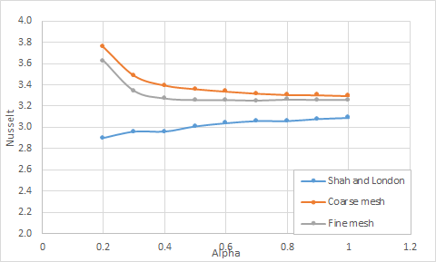
The following table and figure present the comparison of the average Nusselt numbers predicted by the solver with the theory of Shah and London [51] for constant wall flux.
| α* | Nucorr | Nucoarse | Errorcoarse (%) | Nufine | Errorfine (%) |
|---|---|---|---|---|---|
| 0.2 | 2.9 | 3.7583 | 29.60 | 3.6229 | 24.92 |
| 0.3 | 2.96 | 3.4876 | 17.83 | 3.3410 | 12.87 |
| 0.4 | 2.96 | 3.3952 | 14.70 | 3.2705 | 10.49 |
| 0.5 | 3.01 | 3.3603 | 11.64 | 3.2554 | 8.15 |
| 0.6 | 3.04 | 3.3376 | 9.79 | 3.2560 | 7.10 |
| 0.7 | 3.06 | 3.3182 | 8.44 | 3.2503 | 6.22 |
| 0.8 | 3.06 | 3.3052 | 8.01 | 3.2601 | 6.54 |
| 0.9 | 3.08 | 3.3032 | 7.24 | 3.2561 | 5.72 |
| 1.0 | 3.09 | 3.2948 | 6.63 | 3.2567 | 5.39 |

