VVC4 - Natural convection through two vertical parallel plates
| Gap (m) | W (m) | H/S | Boundary condition | Test case |
|---|---|---|---|---|
| 0.01 | 1 | 5 | Case A: Temperature constraint | SVTEST29 |
| 0.01 | 1 | 5 | Case B: Heat flux load | SVTEST30 |
| 0.01 | 1 | 10 | Case A: Temperature constraint | SVTEST31 |
| 0.01 | 1 | 10 | Case B: Heat flux load | SVTEST32 |
| 0.01 | 1 | 20 | Case A: Temperature constraint | SVTEST33 |
| 0.01 | 1 | 20 | Case B: Heat flux load | SVTEST34 |
| 0.01 | 1 | 40 | Case A: Temperature constraint | SVTEST35 |
| 0.01 | 1 | 40 | Case B: Heat flux load | SVTEST36 |
| 0.01 | 1 | 70 | Case A: Temperature constraint | SVTEST37 |
| 0.01 | 1 | 70 | Case B: Heat flux load | SVTEST38 |
| 0.01 | 1 | 100 | Case A: Temperature constraint | SVTEST39 |
| 0.01 | 1 | 100 | Case B: Heat flux load | SVTEST40 |
| 0.025 | 2.5 | 5 | Case A: Temperature constraint | SVTEST41 |
| 0.025 | 2.5 | 10 | Case A: Temperature constraint | SVTEST42 |
| 0.025 | 2.5 | 20 | Case A: Temperature constraint | SVTEST43 |
| 0.025 | 2.5 | 20 | Case B: Heat flux load | SVTEST44 |
| 0.025 | 2.5 | 40 | Case A: Temperature constraint | SVTEST45 |
| 0.025 | 2.5 | 40 | Case B: Heat flux load | SVTEST46 |
| 0.025 | 2.5 | 70 | Case A: Temperature constraint | SVTEST47 |
| 0.025 | 2.5 | 70 | Case B: Heat flux load | SVTEST48 |
| 0.025 | 2.5 | 100 | Case A: Temperature constraint | SVTEST49 |
| 0.025 | 2.5 | 100 | Case B: Heat flux load | SVTEST50 |
| 0.05 | 5 | 5 | Case A: Temperature constraint | SVTEST51 |
| 0.05 | 5 | 10 | Case A: Temperature constraint | SVTEST52 |
| 0.05 | 5 | 20 | Case A: Temperature constraint | SVTEST53 |
| 0.05 | 5 | 40 | Case A: Temperature constraint | SVTEST54 |
| 0.05 | 5 | 70 | Case A: Temperature constraint | SVTEST55 |
| 0.05 | 5 | 100 | Case A: Temperature constraint | SVTEST56 |
Description
The purpose of this verification test is to correlate the heat transfer away from two parallel plates, as quantified by the Nusselt number, with the ratio of buoyancy to viscosity, as quantified by the Rayleigh number. The mechanism for heat transfer is natural convection. Two test cases are considered: one where the plates have fixed temperatures, the other where the plates have fixed heat fluxes, as summarized in the table below. The Rayleigh number is varied by changing the height (H) of the plates, and the gap (S) between the plates.
| Case | Description | Plate 1 | Plate 2 |
|---|---|---|---|
| A | Constant plate temperatures | T1 = 100 °C | T1 = 30 °C |
| B | Constant plate heat fluxes | q"1= 400 W/m2 | q"2 = 100 W/m2 |
Geometry
A solid block geometry represents the fluid domain between two vertical parallel plates. The X dimension is the width (W) the Y dimension is the gap (S), and the Z dimension is the height (H) as shown in the figure below. These three parameters are related as follows:
where, to vary the geometry, S ∈ [0.01, 0.025, 0.05] m and C ∈ [5, 10, 20, 40, 70, 100].
Simulation model
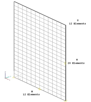
The geometry is meshed using linear hexahedral elements. The following mesh controls are used:
- Height: 20 elements
- Width: 12 elements
- Length: 12 elements
The following figure shows the generated mesh.

The solid mesh is assigned the following fluid properties (air):
- Mass density: ρ = 1.207kg/m3
- Thermal conductivity: k = 0.0263W/m · K
- Thermal expansion coefficient: β = 3.41 × 10⁻³ K−1
- Specific heat at constant pressure: Cp = 1007J/kg · K
- Gas constant: R = 287J/kg · K
- Dynamic viscosity: µ = 1.85 × 10⁻⁵ kg/m · s
The following boundary conditions are applied:
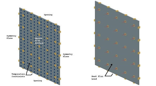
- Flow Surface: Boundary Flow Surface on the faces parallel to the XZ plane using the No Slip Wall option with smooth wall friction and convection properties set to automatic
- Flow Boundary Condition: Opening on the faces parallel to the XY plane
- Symmetry Plane on the remaining faces parallel to the YZ plane
- Temperature constraint (Case A) on the one plate side with a value of T = 100 ºC and on the opposite plate side with a value of T = 30 °C
- Thermal Loads: Heat Flux (Case B) on the one plate side with a q"1= 400 W/m2 and on the opposite plate side with a q"2 = 100 W/m2

This model uses Advanced Thermal-Flow solution type with the following options:
- Turbulence Model: None (Laminar Flow)
- Solution Type: Steady State
- Ambient Conditions: Fluid temperature = 20 °C. The gravity, g, vector is in the negative Z-direction.
- Buoyancy: selected
For solver parameters, on the 3D Flow Solver page, from the Buoyancy Model list, select Boussinesq.
Theory
The average free-convection heat transfer coefficient can typically be represented by the following relationship:
where:
- Nu is the Nusselt number.
- Gr is the Grashof number.
- Pr is the Prandtl number.
- f represents some functional relationship, found experimentally.
The product of the Grashof number and the Prandtl number is the Rayleigh number (Gr·Pr = Ra). For Pr >> 1, fluid buoyancy forces are balanced by fluid viscous forces, and it is found that Nu = f(Ra) [24]. For Pr << 1, fluid buoyancy forces are balanced by dynamic pressure and fluid inertia, and it is found that Nu = f(Ra·Pr) [24]. The Nusselt number is the non-dimensional ratio of convective heat transfer to conductive heat transfer given by:
where:
- h is the convective heat transfer coefficient of the flow.
- L is the characteristic length.
- k is the thermal conductivity of the fluid.
In the case of parallel isothermal plates (case A), the Rayleigh number is:
where:
- ν=μ/ρ is the kinematic viscosity.
- α=k/(ρCp)
- Tw is the average wall temperature of T1 and T2.
The correlation found by Aung et al. [24] is:
where m=–1.9, c=1.2, and Cl=0.515 for air. This correlation is valid for Rayleigh numbers up to around 105. The characteristic length for this problem is S, so the Nusselt number can be calculated by:
where q is the rate of heat transfer to the convecting air, meaning q/(2HW) is the total heat flux.
In the case of parallel plates with uniform heat flux, (case B), the Rayleigh number is non-standard:
where q" is the average heat flux. The correlation found by Aung et al. [24] is:
where m=–3.5, c=1.07, and Hl=0.624 for air [24]. This correlation is valid for Rayleigh numbers up to around 104. In this case, the heat flux is known, so the Nusselt number can be calculated by:
where Tw(½) is the average wall temperature between the two plates, half the distance, H, up the plates.
Results
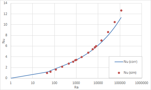
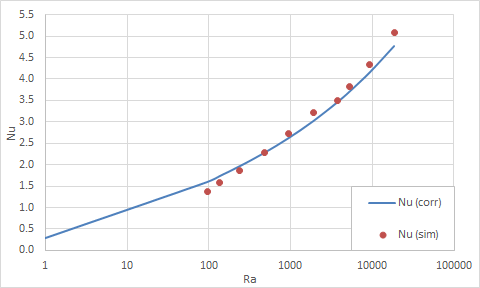
Using a Report simulation object, the total heat transfer from the parallel plates to the convecting air is obtained. Average wall temperatures are obtained through post processing. The tables below compare Nusselt numbers computed from the software results and those numbers predicted by the correlations of Aung et al. [24] The percentage error surpassed 10% for Rayleigh numbers below 200, but there is a good agreement for Rayleigh numbers on the order of 1000 to 10000.
Case A - isothermal parallel plates
| S (m) | H/S | W (m) | Ra | q (W) | Nu (sim) | Nu (corr) | Error (%) |
|---|---|---|---|---|---|---|---|
| 0.01 | 5 | 1 | 906.86 | 39.7 | 3.35 | 3.37 | 0.56 |
| 0.01 | 10 | 1 | 453.43 | 64.5 | 2.72 | 2.81 | 3.07 |
| 0.01 | 20 | 1 | 226.71 | 102 | 2.15 | 2.31 | 6.71 |
| 0.01 | 40 | 1 | 113.36 | 153 | 1.62 | 1.83 | 11.85 |
| 0.01 | 70 | 1 | 64.78 | 200 | 1.21 | 1.45 | 16.57 |
| 0.01 | 100 | 1 | 45.34 | 229 | 0.97 | 1.20 | 19.44 |
| 0.025 | 5 | 2.5 | 14169.66 | 209 | 7.06 | 6.74 | 4.77 |
| 0.025 | 10 | 2.5 | 7084.83 | 342 | 5.78 | 5.67 | 1.96 |
| 0.025 | 20 | 2.5 | 3542.42 | 565 | 4.77 | 4.76 | 0.21 |
| 0.025 | 40 | 2.5 | 1771.21 | 937 | 3.95 | 4.00 | 1.06 |
| 0.025 | 70 | 2.5 | 1012.12 | 1410 | 3.40 | 3.47 | 1.90 |
| 0.025 | 100 | 2.5 | 708.48 | 1840 | 3.11 | 3.16 | 1.73 |
| 0.05 | 5 | 5 | 113357.30 | 748 | 12.64 | 11.34 | 11.47 |
| 0.05 | 10 | 5 | 56678.65 | 1240 | 10.48 | 9.54 | 9.88 |
| 0.05 | 20 | 5 | 28339.33 | 2035 | 8.59 | 8.02 | 7.23 |
| 0.05 | 40 | 5 | 14169.66 | 3334 | 7.04 | 6.74 | 4.46 |
| 0.05 | 70 | 5 | 8096.95 | 4981 | 6.01 | 5.86 | 2.59 |
| 0.05 | 100 | 5 | 5667.87 | 6437 | 5.44 | 5.36 | 1.47 |
Case B - constant flux parallel plates
| S (m) | H/S | W (m) | Ra | T1 (°C) | T2 (°C) | T1/2 (°C) | Nusim | Nucor | Error (%) |
|---|---|---|---|---|---|---|---|---|---|
| 0.01 | 5 | 1 | 1915.6 | 64.95 | 34.28 | 49.62 | 3.21 | 3.02 | 6.23 |
| 0.01 | 10 | 1 | 957.81 | 72.63 | 37.27 | 54.95 | 2.72 | 2.63 | 3.61 |
| 0.01 | 20 | 1 | 478.91 | 81.77 | 41.67 | 61.72 | 2.28 | 2.28 | 0.11 |
| 0.01 | 40 | 1 | 239.45 | 93.18 | 48.54 | 70.86 | 1.87 | 1.96 | 4.88 |
| 0.01 | 70 | 1 | 136.83 | 104.00 | 57.01 | 80.51 | 1.57 | 1.74 | 9.45 |
| 0.01 | 100 | 1 | 95.78 | 114.29 | 64.43 | 89.36 | 1.37 | 1.60 | 14.14 |
| 0.025 | 20 | 2.5 | 18707 | 91.27 | 42.17 | 66.72 | 5.09 | 4.77 | 6.54 |
| 0.025 | 40 | 2.5 | 9353.6 | 103.70 | 45.71 | 74.71 | 4.34 | 4.16 | 4.54 |
| 0.025 | 70 | 2.5 | 5344.9 | 115.28 | 49.07 | 82.18 | 3.82 | 3.71 | 2.90 |
| 0.025 | 100 | 2.5 | 3741.4 | 123.89 | 51.70 | 87.80 | 3.51 | 3.46 | 1.38 |
The following figures plot these comparisons graphically.


